Download
1 / 72
770 likes | 1.01k Views
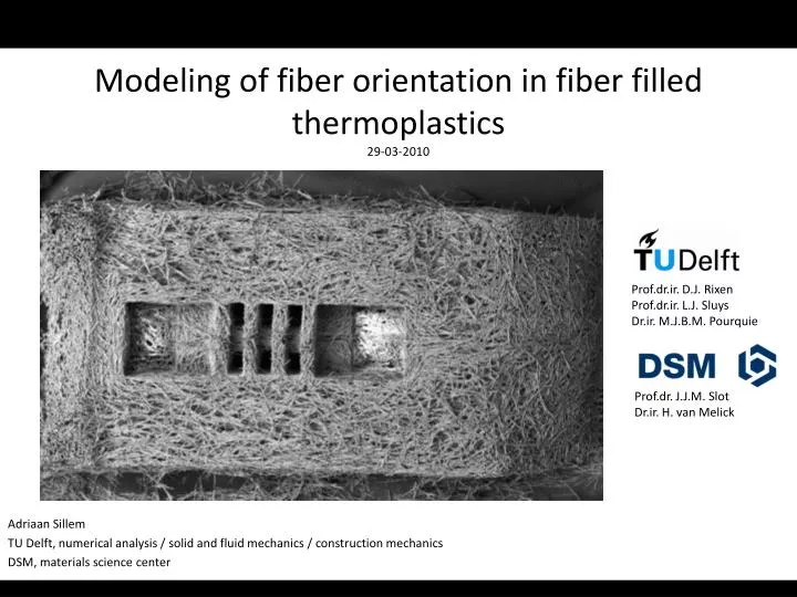
Modeling of fiber orientation in fiber filled thermoplastics 29-03-2010. Prof.dr.ir. D.J. Rixen Prof.dr.ir. L.J. Sluys Dr.ir. M.J.B.M. Pourquie. Adriaan Sillem TU Delft, numerical analysis / solid and fluid mechanics / construction mechanics DSM, materials science center.

E N D
Modeling of fiber orientation in fiber filled thermoplastics 29-03-2010 Prof.dr.ir. D.J. Rixen Prof.dr.ir. L.J. Sluys Dr.ir. M.J.B.M. Pourquie Adriaan Sillem TU Delft, numerical analysis / solid and fluid mechanics / construction mechanics DSM, materials science center Prof.dr. J.J.M. Slot Dr.ir. H. van Melick
Layout Introduction. Application. Models. Test cases. Conclusions and recommendations INTRODUCTION | APPLICATION | MODELS | TEST CASES | CONCLUSIONS AND RECOMMENDATIONS
Introduction INTRODUCTION | APPLICATION | MODELS | TEST CASES | CONCLUSIONS AND RECOMMENDATIONS
Project Master student mechanical engineering. Final project of mechanical engineering study. Carried out at DSM, a Dutch multinational Life Sciences and Materials Sciences company. INTRODUCTION | APPLICATION | MODELS | TEST CASES | CONCLUSIONS AND RECOMMENDATIONS
Interest DSM is interested in simulating the production process injection molding. INTRODUCTION | APPLICATION | MODELS | TEST CASES | CONCLUSIONS AND RECOMMENDATIONS
Objective Implementation of a model to gain insight in the fiber orientation development during injection molding. INTRODUCTION | APPLICATION | MODELS | TEST CASES | CONCLUSIONS AND RECOMMENDATIONS
Contribution Reproduction of literature material. Implementation of models. Interpretation of output. Comparison of quality of approximations. Instruction of implementation. Integration of all of the former in a report. INTRODUCTION | APPLICATION | MODELS | TEST CASES | CONCLUSIONS AND RECOMMENDATIONS
Application INTRODUCTION | APPLICATION | MODELS | TEST CASES | CONCLUSIONS AND RECOMMENDATIONS
Thermoplastic products Focus of the project is on thermoplastic products. In our daily lives, we encounter thermoplastic products. INTRODUCTION | APPLICATION | MODELS | TEST CASES | CONCLUSIONS AND RECOMMENDATIONS
Thermoplastic products Examples INTRODUCTION | APPLICATION | MODELS | TEST CASES | CONCLUSIONS AND RECOMMENDATIONS
Material Used materials in granules or pellets form. INTRODUCTION | APPLICATION | MODELS | TEST CASES | CONCLUSIONS AND RECOMMENDATIONS
Injection molding INTRODUCTION | APPLICATION | MODELS | TEST CASES | CONCLUSIONS AND RECOMMENDATIONS
Material Used materials in granules or pellets form. INTRODUCTION | APPLICATION | MODELS | TEST CASES | CONCLUSIONS AND RECOMMENDATIONS
Material Add discontinuous fibers to improve the quality of the final product. Glass or carbon fibers, for instance. Influences: viscosity, stiffness, thermal conductivity and electrical conductivity. DSM wants to control these properties. INTRODUCTION | APPLICATION | MODELS | TEST CASES | CONCLUSIONS AND RECOMMENDATIONS
Material Typical volume fractions are 8-30%. Typical weight fractions 15-60%. Typical average final lengths 200-300 [μm]. Typical diameter 10 [μm]. Average human hair is 100 [μm]. INTRODUCTION | APPLICATION | MODELS | TEST CASES | CONCLUSIONS AND RECOMMENDATIONS
Configuration of the fibers Configuration of the fibers. INTRODUCTION | APPLICATION | MODELS | TEST CASES | CONCLUSIONS AND RECOMMENDATIONS
Configuration of the fibers How is the configuration of the fibers controlled? We want to control the production process. INTRODUCTION | APPLICATION | MODELS | TEST CASES | CONCLUSIONS AND RECOMMENDATIONS
Control Configuration of the fibers can be controlled by processing settings on the injection molding machine and mold geometry (expensive!). Simulations are preferred. INTRODUCTION | APPLICATION | MODELS | TEST CASES | CONCLUSIONS AND RECOMMENDATIONS
Software DSM already uses the commercial software Moldflow and Moldex3D to simulate injection molding processes. Problems encountered by DSM: results warpage (kromtrekking) analyses not good, results fiber orientation analyses not good, ‘company secrecy’ response concerning the code, models not up to date. INTRODUCTION | APPLICATION | MODELS | TEST CASES | CONCLUSIONS AND RECOMMENDATIONS
Project DSM wants implementations of the latest fiber orientation models. INTRODUCTION | APPLICATION | MODELS | TEST CASES | CONCLUSIONS AND RECOMMENDATIONS
Fiber orientation How can the configuration of the fibers be described? Location of the fibers. Orientation of the fibers. It is reasonable to assume that the concentration of the fibers in the final product is uniform by approximation. The orientation of the fibers influences the material properties the most. We will focus on the modeling of the orientation. INTRODUCTION | APPLICATION | MODELS | TEST CASES | CONCLUSIONS AND RECOMMENDATIONS
Models INTRODUCTION | APPLICATION | MODELS | TEST CASES | CONCLUSIONS AND RECOMMENDATIONS
Physics behind fiber orientation What are the physics behind the fiber orientation? What are the characteristics? Inertia forces are negligible <-> low Reynolds number. Viscous forces <-> lift and drag. Stiffness of the fibers <-> internal stresses. Fiber-fiber interaction <-> fibers ‘hit’ each other. Fibers influence surrounding flow field <-> coupling of orientation and velocity. Order of increasing complexity of the models. INTRODUCTION | APPLICATION | MODELS | TEST CASES | CONCLUSIONS AND RECOMMENDATIONS
Incompressible homogeneous flow fields Models are constructed for incompressible homogeneous flows. Such flows are characterized by velocities whereof the change in space is constant. The velocity can be described as Incompressibility demands that INTRODUCTION | APPLICATION | MODELS | TEST CASES | CONCLUSIONS AND RECOMMENDATIONS
Incompressible homogeneous flow fields Examples are the simple shear flow field the uniaxial elongational flow field INTRODUCTION | APPLICATION | MODELS | TEST CASES | CONCLUSIONS AND RECOMMENDATIONS
Layout models INTRODUCTION | APPLICATION | MODELS | TEST CASES | CONCLUSIONS AND RECOMMENDATIONS
Jeffery’s equation Ellipsoidal particle immersed in a viscosity dominated fluid INTRODUCTION | APPLICATION | MODELS | TEST CASES | CONCLUSIONS AND RECOMMENDATIONS
Jeffery’s equation INTRODUCTION | APPLICATION | MODELS | TEST CASES | CONCLUSIONS AND RECOMMENDATIONS
Jeffery’s equation INTRODUCTION | APPLICATION | MODELS | TEST CASES | CONCLUSIONS AND RECOMMENDATIONS
Jeffery’s equation Balance between viscous stresses from the flow field and internal stresses of the fiber leads to The re is the aspect ratio of the ellipsoidal particle. The ξ is a function of this aspect ratio. INTRODUCTION | APPLICATION | MODELS | TEST CASES | CONCLUSIONS AND RECOMMENDATIONS
Layout models INTRODUCTION | APPLICATION | MODELS | TEST CASES | CONCLUSIONS AND RECOMMENDATIONS
Folgar-Tucker model Model fiber-fiber interaction deterministically or stochastically? INTRODUCTION | APPLICATION | MODELS | TEST CASES | CONCLUSIONS AND RECOMMENDATIONS
Folgar-Tucker model Outcome of a throw of a dice. Hard to say in a deterministic sense. Easy to say in a stochastic (probabilistic) sense. Same holds for fiber-fiber interaction. INTRODUCTION | APPLICATION | MODELS | TEST CASES | CONCLUSIONS AND RECOMMENDATIONS
Folgar-Tucker model Three equations, four unknowns, not solvable. INTRODUCTION | APPLICATION | MODELS | TEST CASES | CONCLUSIONS AND RECOMMENDATIONS
Folgar-Tucker model INTRODUCTION | APPLICATION | MODELS | TEST CASES | CONCLUSIONS AND RECOMMENDATIONS
Folgar-Tucker model Four equations, four unknowns, so solvable. INTRODUCTION | APPLICATION | MODELS | TEST CASES | CONCLUSIONS AND RECOMMENDATIONS
Folgar-Tucker model Viscous and internal stresses of a convective nature. Fiber-fiber interaction of a diffusive nature. INTRODUCTION | APPLICATION | MODELS | TEST CASES | CONCLUSIONS AND RECOMMENDATIONS
Jeffery’s equation INTRODUCTION | APPLICATION | MODELS | TEST CASES | CONCLUSIONS AND RECOMMENDATIONS
Partial information Solving the probability density is very demanding in the computational sense. Is there a computationally less expensive approach? INTRODUCTION | APPLICATION | MODELS | TEST CASES | CONCLUSIONS AND RECOMMENDATIONS
Layout models INTRODUCTION | APPLICATION | MODELS | TEST CASES | CONCLUSIONS AND RECOMMENDATIONS
Partial information --> less information • The only unknowns are the orientation tensors • Sum is infinite! Maybe a set of lower order terms already give enough information on the fiber orientation. INTRODUCTION | APPLICATION | MODELS | TEST CASES | CONCLUSIONS AND RECOMMENDATIONS
Partial information • Let us first consider the symmetric second order tensor. p3p3 sin θ p1p1 sin θ p2p2 sin θ p2p3 sin θ p1p2 sin θ p1p3 sin θ INTRODUCTION | APPLICATION | MODELS | TEST CASES | CONCLUSIONS AND RECOMMENDATIONS
Partial information The orientation tensor already gives sufficient information on the fiber orientation. But can it be solved more efficiently? INTRODUCTION | APPLICATION | MODELS | TEST CASES | CONCLUSIONS AND RECOMMENDATIONS
Folgar-Tucker tensor form • The rate equation for A. • Not a function of orientation p. Only of time t. • We have realized a reduction of the #DOF from three to one. The tensor form can be solved more efficiently. INTRODUCTION | APPLICATION | MODELS | TEST CASES | CONCLUSIONS AND RECOMMENDATIONS
Folgar-Tucker tensor form • The rate equation for A. Comparison with experimental results show that the transient time is too short. INTRODUCTION | APPLICATION | MODELS | TEST CASES | CONCLUSIONS AND RECOMMENDATIONS
Layout models INTRODUCTION | APPLICATION | MODELS | TEST CASES | CONCLUSIONS AND RECOMMENDATIONS
Correction We need to ‘correct’ the rate equation. How should we do this? INTRODUCTION | APPLICATION | MODELS | TEST CASES | CONCLUSIONS AND RECOMMENDATIONS
Correction A straightforward way would be Model is not objective. INTRODUCTION | APPLICATION | MODELS | TEST CASES | CONCLUSIONS AND RECOMMENDATIONS
Wang-O’Gara-Tucker In 2008, Wang, O’Gara and Tucker found a way to prolong the transient time in an objective way. Because the orientation tensor is symmetric, it has a spectral decomposition. INTRODUCTION | APPLICATION | MODELS | TEST CASES | CONCLUSIONS AND RECOMMENDATIONS
Wang-O’Gara-Tucker Is objective! But the equation is not solvable. INTRODUCTION | APPLICATION | MODELS | TEST CASES | CONCLUSIONS AND RECOMMENDATIONS