Download
1 / 55
560 likes | 766 Views
IASI Principal Components – Experiences at EUMETSAT . Tim.Hultberg@EUMETSAT.INT. Operational IASI PC scores. Noise normalisation. Suppression of instrument effects. Use of reconstructed radiances in IASI L2. Channel selection for reconstructed radiances.

E N D
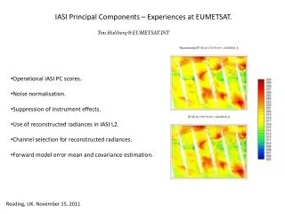
IASI Principal Components – Experiences at EUMETSAT. Tim.Hultberg@EUMETSAT.INT • Operational IASI PC scores. • Noise normalisation. • Suppression of instrument effects. • Use of reconstructed radiances in IASI L2. • Channel selection for reconstructed radiances. • Forward model error mean and covariance estimation. Reading, UK. November 15, 2011
http://www.eumetsat.int/Home/Main/DataProducts/Resources IASI Level 1 PCC Product Generation Specification, EUM.OPS-EPS.SPE.08.0199 IASI Level 1 PCC Product Format Specification, EUM.OPS-EPS.SPE.08.0195 IASI Principal Component Compression (IASI PCC) FAQ Dissemination of IASI PC scores on EUMETCast started August 2010 and was declared operational February 2011 Since 2010.08.05 (demonstrational status): IASI PCC Eigenvector files - Band 1,2 and 3 (HDF5) 1.3 EPS Product Validation Report: IASI L1 PCC PPF (Part 1), EUM/OPS-EPS/REP/10/0148 Since 2011.02.22 (operational status): IASI PCC Eigenvector files - Band 1,2 and 3 (HDF5) 1.4 EPS Product Validation Report: IASI L1 PCC PPF (Part 2), EUM/OPS-EPS/REP/11/0036 Collaboration with NWPSAF (Nigel Atkinson, Fiona Hilton). Eigenvectors to be shared with EARS-IASI (AAPP). IASI Principal Component Compression Product and Documentation
Band separation + Compression/decompression is faster - About 40 extra PC scores are needed Band separation Band 1 channel# 0 to 1996 (1997) Band 2 channel# 1997 to 5115 (3119) Band 3 channel# 5116 to 8460 (3345) Band 1: 645.00 – 1144.00 cm-1 Band 2: 1144.25 - 1923.75 cm-1 Band 3: 1924.00 – 2760.00 cm-1
Measured radiances = “true radiances” + noise PC scores Reconstructed radiances (short hand notation) 8461 a projection (a linear transformation P from R to itself such that P2 = P) two orthogonal subspaces providing a unique decomposition of each spectrum range(P) Signal space kernel(P) Noise space
Total Signal Noise Raw radiance Reconstructed radiance (Signal Space) Residual (Noise Space) Raw radiance noise covariance matrix Reconstructed radiance noise covariance matrix Covariance of the residual (in the absence of reconstruction error).
Instrument noise covariance (1040-1090 cm-1) Raw radiances Reconstructed radiances
Ammonia NH3 signal expressed as BT difference between a channel sensitive to NH3 (at 867.75 cm-1) and the average of two nearby window channels (at 861.25 and 873.5cm-1) Coheur et al.: “IASI measurements of reactive trace species in biomass burning plumes”
How many scores? PC scores spatial correlation for 8 orbits at different seasons and areas Band 1: 90 Band 2: 120 Band 3: 80 (now 90) Total : 290
Noise normalisation • Diagonal noise normalisation matrix. • noise does not get de-correlated • it works, but is suboptimal and should be changed (Nigel Atkinson, Fiona Hilton) • N equal to the matrix square root of the instrument noise covariance matrix. • the correlated L1C noise gets normalised and de-correlated. • equivalent to de-apodising prior to compression • ensures that same amount of noise is carried by all eigenvectors No noise normalisation (scaled) Diagonal noise normalisation Full noise normalisation User Feedback Form (please)
Reconstruction score (Noise normalised) residual Reconstruction score (Residual RMS) 3 reconstruction scores (one for each IASI spectral band) are computed and disseminated for each spectrum. High reconstruction score is a sign that part of the atmospheric signal could not be represented in the truncated eigenvector space and is therefore contained in the residual.
Monitoring of noise evolution Decontamination, March 2008
Decontamination, September 2010. Noise reduction of 0 -20% in each channel.
Undetected ‘spikes’ (‘spike’: high-frequency disturbance of the interferogram) Band 1 outliers (threshold 1.2) Band 2 outliers (threshold 1.25) Band 3 outliers (threshold 1.45) South Atlantic Anomaly
Back to normal operation... No history available for deriving filtered calibration coefficients
Photonic noise - increases with the signal Expected noise / reconstruction score depends on the radiance (and the detector)
Russian fires 1-10 August 2010 (a total 70 outliers in the area below)
Residual statistics, one full day (20100321) Max Std Mean Configuration change of L1C processing (‘Gibbs effect’) Min
Residuals, 20090330 Histogram of normalised residual at 820 cm-1
Spatial correlation in residual … 90+120+80 PCs …not much smaller after big (moderate) increase of the number of PCs 90+120+80 PCs minus 300+300+300 PCs 300+300+300 PCs
Band 1, PCC noise estimation, First iteration • Noise guess • Noise in residual • Reconstructed noise • New noise estimate W/m2/sr/m-1 Wavenumber (cm-1) Part of the instrument noise is contained in signal space, the rest in the residuals. All we have to do is to add the two together. Noise in residual can be estimated directly (assuming no reconstruction error) Noise in signal estimated by transformation of first guess of full noise
Band 1, PCC noise estimation, Second iteration • Noise guess • Noise in residual • Reconstructed noise • New noise estimate W/m2/sr/m-1 Wavenumber (cm-1)
Band 2, PCC noise estimation, First iteration • Noise guess • Noise in residual • Reconstructed noise • New noise estimate W/m2/sr/m-1 Wavenumber (cm-1)
Band 2, PCC noise estimation, Second iteration • Noise guess • Noise in residual • Reconstructed noise • New noise estimate W/m2/sr/m-1 Wavenumber (cm-1)
Practical issues • Execution speed • Compress/reconstruct many spectra simultaneously, i.e. use matrix-matrix multiplications instead of matrix-vector multiplications • and can be pre-computed • No execution time penalty for using non-diagonal N / • Quantisation of PC scores • Dynamic range of PC scores decreases with the rank, most scores can be stored in one byte • Use update formulas for covariance matrix • when adding outlier spectra to the training set
EUMETSAT IASI L2 1DVar RTTOV-10 since 20/10 2011 (RTIASI-4 before) State-vector representation: T: 28 PC scores 101 (K) W: 18 PC scores 101 (log(ppmv)) O: 9 PC scores 101 (log(ppmv)) Ts: (K) One fixed global a priori (mean and covariance) Forecast used for cloud screening, but not in retrieval 316 channels in band 1 and 2 (subset of the 366 ‘ECMWF-channels’) Measurement space: Reconstructed radiances converted to BT Full observation error covariance matrix based on OBS-CALC (diagonal multiplied by 1.03 to make it invertible). Object oriented. Abstract interfaces: SquareMatrix >> PDMatrix / DiagonalMatrix Frtm >> frtm_rttov_iasi / frtm_rtiasi / Frtm_composed(&Frtm, &Statevector) Statevector >> Statevector_TWO mfunction >> cost_function(&SquareMatrix, &Frtm)
Instead of inflating the diagonal of the observation error covariance matrix, we can limit the number of reconstructed channels to the number of PCs (and get the same results as when doing the retrieval in PC space) Matrix of s leading eigenvectors (rank s) Can always choose s linearly independent rows of E (i.e. such that is invertible) Subset of reconstructed (noise normalised) radiances = = where Subset of channels should be chosen to minimise the condition number of in practise we can use a heuristic to find a channel subset with low cond( )
Channel selection heuristic Start with X = E (m x s matrix of s most significant eigenvectors) Repeat s times: Pick the row in X with largest norm From all rows in X, subtract its projection onto the direction of the chosen row X = E(1:m,1:s) Cs = {} For j=1 to s i = argmax{ norm(Xi) : i=1,...,m} Cs += {i} For k=1 to m Xk -= (Xk·Xi / Xi·Xi) Xi End End Not ‘monotone’, i.e. Cs not necessarily a subset of Cs+1 (if this is wanted we should consider only the first j columns when computing the norm in step a)
Band 1. Channel selection. Rows: channels (1 to 1997) Cols: PC rank (1 to 90)
Forward model error mean and covariance estimation • Synthetic spectra (RTTOV-10) often have higher reconstruction scores than real data. • i.e. is far from zero • (this could be avoided with a PCRTM with eigenvectors corresponding to signal space) In the next slides we look at using the Chevallier profiles and RTTOV-10 for 15 different scan angles. The contribution of to the forward model error can be estimated by projecting real data onto Forward model space (i.e. using eigenvectors based on synthetic spectra) (or by forward propagation of variability of state-vector elements not being retrieved)
Band 1 Mean( ) Std( )


![Planning Adaptive Interfaces [RWD Summit 2016]](https://cdn4.slideserve.com/7568466/planning-adaptive-interfaces-dt.jpg)