Introduction to Parallel Processing
590 likes | 605 Views
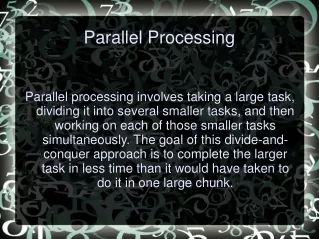
This introduction explores the fundamentals of parallel computing, including parallel computer architecture, performance goals, and the feasibility of implementing parallel systems. It delves into topics such as Flynn’s classification of computer architecture, parallel programming models, and current trends in parallel architectures. The text covers the need for parallel computing driven by application demands and technology trends like chip-multiprocessors. Factors affecting parallel system performance and scalability goals are also discussed, providing a comprehensive overview of the landscape of parallel processing.

Introduction to Parallel Processing
E N D
Presentation Transcript
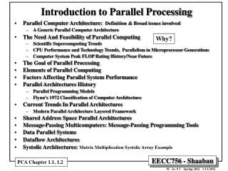
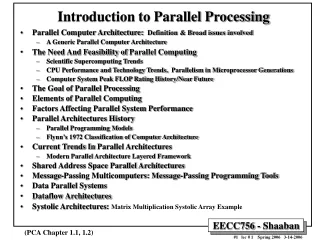
Introduction to Parallel Processing • Parallel Computer Architecture: Definition & Broad issues involved • A Generic Parallel Computer Architecture • The Need And Feasibility of Parallel Computing • Scientific Supercomputing Trends • CPU Performance and Technology Trends, Parallelism in Microprocessor Generations • Computer System Peak FLOP Rating History/Near Future • The Goal of Parallel Processing • Elements of Parallel Computing • Factors Affecting Parallel System Performance • Parallel Architectures History • Parallel Programming Models • Flynn’s 1972 Classification of Computer Architecture • Current Trends In Parallel Architectures • Modern Parallel Architecture Layered Framework • Shared Address Space Parallel Architectures • Message-Passing Multicomputers: Message-Passing Programming Tools • Data Parallel Systems • Dataflow Architectures • Systolic Architectures: Matrix MultiplicationSystolic Array Example (PCA Chapter 1.1, 1.2)
Parallel Computer Architecture A parallel computer (or multiple processor system) is a collection of communicating processing elements (processors) that cooperate to solve large computational problems fast by dividing such problems into parallel tasks, exploiting Thread-Level Parallelism (TLP). • Broad issues involved: • The concurrency and communication characteristics of parallel algorithms for a given computational problem (represented by dependency graphs) • Computing Resources and Computation Allocation: • The number of processing elements (PEs), computing power of each element and amount/organization of physical memory used. • What portions of the computation and data are allocated or mapped to each PE. • Data access, Communication and Synchronization • How the processing elements cooperate and communicate. • How data is shared/transmitted between processors. • Abstractions and primitives for cooperation/communication. • The characteristics and performance of parallel system network (System interconnects). • Parallel Processing Performance and Scalability Goals: • Maximize performance enhancement of parallelism: Maximize Speedup. • By minimizing parallelization overheads and balancing workload on processors • Scalability of performance to larger systems/problems. i.e Parallel Processing Processor = Programmable computing element that runs stored programs written using pre-defined instruction set Processing Elements = PEs = Processors
A Generic Parallel Computer Architecture Parallel Machine Network (Custom or industry standard) A processing node Processing Nodes Network Interface (custom or industry standard) Operating System Parallel Programming Environments One or more processing elements or processors per node: Custom or commercial microprocessors. Single or multiple processors per chip Processing Nodes: Each processing node contains one or more processing elements (PEs) or processor(s), memory system, plus communication assist: (Network interface and communication controller) Parallel machine network (System Interconnects). Function of a parallel machine network is to efficiently (reduce communication cost) transfer information (data, results .. ) from source node to destination node as needed to allow cooperation among parallel processing nodes to solve large computational problems divided into a number parallel computational tasks. Parallel Computer = Multiple Processor System
The Need And Feasibility of Parallel Computing Driving Force • Application demands: More computing cycles/memory needed • Scientific/Engineering computing: CFD, Biology, Chemistry, Physics, ... • General-purpose computing: Video, Graphics, CAD, Databases, Transaction Processing, Gaming… • Mainstream multithreaded programs, are similar to parallel programs • Technology Trends: • Number of transistors on chip growing rapidly. Clock rates expected to continue to go up but only slowly. Actual performance returns diminishing due to deeper pipelines. • Increased transistor density allows integrating multiple processor cores per creating Chip-Multiprocessors (CMPs) even for mainstream computing applications (desktop/laptop..). • Architecture Trends: • Instruction-level parallelism (ILP) is valuable (superscalar, VLIW) but limited. • Increased clock rates require deeper pipelines with longer latencies and higher CPIs. • Coarser-level parallelism (at the task or thread level, TLP), utilized in multiprocessor systems is the most viable approach to further improve performance. • Main motivation for development of chip-multiprocessors (CMPs) • Economics: • The increased utilization of commodity of-the-shelf (COTS) components in high performance parallel computing systems instead of costly custom components used in traditional supercomputers leading to much lower parallel system cost. • Today’s microprocessors offer high-performance and have multiprocessor support eliminating the need for designing expensive custom Pes. • Commercial System Area Networks (SANs) offer an alternative to custom more costly networks
Why is Parallel Processing Needed?Challenging Applications in Applied Science/Engineering • Astrophysics • Atmospheric and Ocean Modeling • Bioinformatics • Biomolecular simulation: Protein folding • Computational Chemistry • Computational Fluid Dynamics (CFD) • Computational Physics • Computer vision and image understanding • Data Mining and Data-intensive Computing • Engineering analysis (CAD/CAM) • Global climate modeling and forecasting • Material Sciences • Military applications • Quantum chemistry • VLSI design • …. Such applications have very high computational and memory requirements that cannot be met with single-processor architectures. Many applications contain a large degree of computational parallelism Driving force for High Performance Computing (HPC) and multiple processor system development
Why is Parallel Processing Needed?Scientific Computing Demands (Memory Requirement) Computational and memory demands exceed the capabilities of even the fastest current uniprocessor systems 3-5 GFLOPS for uniprocessor
Scientific Supercomputing Trends • Proving ground and driver for innovative architecture and advanced high performance computing (HPC) techniques: • Market is much smaller relative to commercial (desktop/server) segment. • Dominated by costly vector machines starting in the 70s through the 80s. • Microprocessors have made huge gains in the performance needed for such applications: • High clock rates. (Bad: Higher CPI?) • Multiple pipelined floating point units. • Instruction-level parallelism. • Effective use of caches. • Multiple processor cores/chip (2 cores 2002-2005, 4 end of 2006, 8 cores 2007?) However even the fastest current single microprocessor systems still cannot meet the needed computational demands. • Currently: Large-scale microprocessor-based multiprocessor systems and computer clusters are replacing (replaced?) vector supercomputers that utilize custom processors. Enabled with high transistor density/chip As shown in last slide
Uniprocessor Performance Evaluation • CPU Performance benchmarking is heavily program-mix dependent. • Ideal performance requires a perfect machine/program match. • Performance measures: • Total CPU time = T = TC / f = TC x C = Ix CPI x C = I x (CPIexecution+ m x k) xC (in seconds) TC = Total program execution clock cycles f = clock rate C = CPU clock cycle time = 1/f I = Instructions executed count CPI = Cycles per instruction CPIexecution = CPI with ideal memory m = Memory stall cycles per memory access k = Memory accesses per instruction • MIPS Rating = I / (T x 106) = f / (CPI x 106) = f x I /(TC x 106) (in million instructions per second) • Throughput Rate: Wp = 1/ T = f /(I x CPI) = (MIPS) x 106 /I (in programs per second) • Performance factors: (I, CPIexecution, m, k, C) are influenced by: instruction-set architecture (ISA) , compiler design, CPU micro-architecture, implementation and control, cache and memory hierarchy, program access locality, and program instruction mix and instruction dependencies. T = I x CPI x C
Single CPU Performance Trends • The microprocessor is currently the most natural building block for • multiprocessor systems in terms of cost and performance. • This is even more true with the development of cost-effective multi-core • microprocessors that support TLP at the chip level.
10,000 100 Intel Processor freq IBM Power PC scales by 2X per DEC generation Gate delays/clock 21264S 1,000 21164A 21264 Pentium(R) 21064A Gate Delays/ Clock Mhz 10 21164 II 21066 MPC750 604 604+ Pentium Pro 100 (R) 601, 603 Pentium(R) 486 386 10 1 1987 1989 1991 1993 1995 1997 1999 2001 2003 2005 Microprocessor Frequency Trend Realty Check: Clock frequency scaling is slowing down! (Did silicone finally hit the wall?) Why? 1- Power leakage 2- Clock distribution delays Result: Deeper Pipelines Longer stalls Higher CPI (lowers effective performance per cycle) ? • Frequency doubles each generation • Number of gates/clock reduce by 25% • Leads to deeper pipelines with more stages • (e.g Intel Pentium 4E has 30+ pipeline stages) Solution: Exploit TLP at the chip level, Chip-multiprocessor (CMPs) T = I x CPI x C
Transistor Count Growth Rate Currently > 1.5 Billion Moore’s Law: 2X transistors/Chip Every 1.5 years (circa 1970) still holds Enables Thread-Level Parallelism (TLP) at the chip level: Chip-Multiprocessors (CMPs) + Simultaneous Multithreaded (SMT) processors Solution • One billion transistors/chip reached in 2005 • Transistor count grows faster than clock rate: Currently ~ 40% per year • Single-threaded uniprocessors do not efficiently utilize the increased transistor count. Limited ILP, increased size of cache
Parallelism in Microprocessor VLSI Generations (ILP) (TLP) Superscalar /VLIW CPI <1 Multiple micro-operations per cycle (multi-cycle non-pipelined) Simultaneous Multithreading SMT: e.g. Intel’s Hyper-threading Chip-Multiprocessors (CMPs) e.g IBM Power 4, 5 Intel Pentium D, Core Duo AMD Athlon 64 X2 Dual Core Opteron Sun UltraSparc T1 (Niagara) Single-issue Pipelined CPI =1 Not Pipelined CPI >> 1 Chip-Level Parallel Processing Even more important due to slowing clock rate increase Single Thread Improving microprocessor generation performance by exploiting more levels of parallelism
Current Dual-Core Chip-Multiprocessor Architectures Two Dice – Shared Package Private Caches Private System Interface Single Die Private Caches Shared System Interface Single Die Shared L2 Cache Cores communicate using shared cache (Lowest communication latency) Examples: IBM POWER4/5 Intel Pentium Core Duo (Yonah), Conroe Sun UltraSparc T1 (Niagara) Cores communicate using on-chip Interconnects (shared system interface) Examples: AMD Dual Core Opteron, Athlon 64 X2 Intel Itanium2 (Montecito) Cores communicate over external Front Side Bus (FSB) (Highest communication latency) Example: Intel Pentium D Source: Real World Technologies, http://www.realworldtech.com/page.cfm?ArticleID=RWT101405234615
Microprocessors Vs. Vector Processors Uniprocessor Performance: LINPACK Now about 3-5 GFLOPS per microprocessor Vector Processors 1 GFLOP (109 FLOPS) Microprocessors
Parallel Performance: LINPACK Current Top LINPACK Performance: Now about 280,600 GFLOPS = 280.6 TeraFLOPS IBM BlueGene/L 131072 (128K) processors (0.7 GHz PowerPC 440) 1 TeraFLOP (1012 FLOPS = 1000 GFLOPS) Current ranking of top 500 parallel supercomputers in the world is found at: www.top500.org
Why is Parallel Processing Needed?LINPAK Performance Trends 1 TeraFLOP (1012 FLOPS =1000 GFLOPS) 1 GFLOP (109 FLOPS) Parallel System Performance Uniprocessor Performance
Computer System Peak FLOP Rating History/Near Future Current Top Peak FP Performance: Now about 367,000 GFLOPS = 367 TeraFLOPS = 0.367 Peta FLOP IBM BlueGene/L 131072 (128K) processors (0.7 GHz PowerPC 440) Peta FLOP (1015 FLOPS = 1000 Tera FLOPS) Teraflop (1012 FLOPS = 1000 GFLOPS)
Time (1 processor) Time (p processors) Performance (p processors) Performance (1 processor) The Goal of Parallel Processing • Goal of applications in using parallel machines: Maximize Speedup over single processor performance Speedup (p processors) = • For a fixed problem size (input data set), performance = 1/time Speedup fixed problem (p processors) = • Ideal speedup = number of processors = p Very hard to achieve Due to parallelization overheads: communication cost, dependencies ...
Sequential Work on one processor Time(1) Speedup = Time(p) Max (Work + Synch Wait Time + Comm Cost + Extra Work) < The Goal of Parallel Processing • Parallel processing goal is to maximize parallel speedup: • Ideal Speedup = p number of processors • Very hard to achieve: Implies no parallelization overheads and perfect load balance among all processors. • Maximize parallel speedup by: • Balancing computations on processors (every processor does the same amount of work) and the same amount of overheads. • Minimizing communication cost and other overheads associated with each step of parallel program creation and execution. • Performance Scalability: Achieve a good speedup for the parallel application on the parallel architecture as problem size and machine size (number of processors) are increased. Parallelization overheads i.e the processor with maximum execution time 1 2
Computing Problems High-level Languages Hardware Architecture Algorithms and Data Structures Operating System Applications Software Performance Evaluation Elements of Parallel Computing Assign parallel computations to processors Mapping Programming Dependency analysis Binding (Compile, Load) e.g Speedup
Elements of Parallel Computing • Computing Problems: • Numerical Computing: Science and and engineering numerical problems demand intensive integer and floating point computations. • Logical Reasoning: Artificial intelligence (AI) demand logic inferences and symbolic manipulations and large space searches. • Parallel Algorithms and Data Structures • Special algorithms and data structures are needed to specify the computations and communication present in computing problems (from dependency analysis). • Most numerical algorithms are deterministic using regular data structures. • Symbolic processing may use heuristics or non-deterministic searches. • Parallel algorithm development requires interdisciplinary interaction. Driving Force
Elements of Parallel Computing • Hardware Resources • Processors, memory, and peripheral devices (processing nodes) form the hardware core of a computer system. • Processor connectivity (system interconnects, network), memory organization, influence the system architecture. • Operating Systems • Manages the allocation of resources to running processes. • Mapping to match algorithmic structures with hardware architecture and vice versa: processor scheduling, memory mapping, interprocessor communication. • Parallelism exploitation possible at: algorithm design, program writing, compilation, and run time.
Elements of Parallel Computing • System Software Support • Needed for the development of efficient programs in high-level languages (HLLs.) • Assemblers, loaders. • Portable parallel programming languages • User interfaces and tools. • Compiler Support • Preprocessor compiler: Sequential compiler and low-level library of the target parallel computer. • Precompiler: Some program flow analysis, dependence checking, limited optimizations for parallelism detection. • Parallelizing compiler: Can automatically detect parallelism in source code and transform sequential code into parallel constructs.
Programmer Programmer Source code written in concurrent dialects of C, C++ FORTRAN, LISP .. Source code written in sequential languages C, C++ FORTRAN, LISP .. Concurrency preserving compiler Parallelizing compiler Concurrent object code Parallel object code Execution by runtime system Execution by runtime system Approaches to Parallel Programming (a) Implicit Parallelism (b) Explicit Parallelism
Factors Affecting Parallel System Performance i.e Inherent Parallelism • Parallel Algorithm Related: • Available concurrency and profile, grain size, uniformity, patterns. • Dependencies between computations represented by dependency graph • Required communication/synchronization, uniformity and patterns. • Data size requirements. • Communication to computation ratio (C-to-C ratio, lower is better). • Parallel program Related: • Programming model used. • Resulting data/code memory requirements, locality and working set characteristics. • Parallel task grain size. • Assignment of tasks to processors: Dynamic or static. • Cost of communication/synchronization primitives. • Hardware/Architecture related: • Total CPU computational power available. • Types of computation modes supported. • Shared address space Vs. message passing. • Communication network characteristics (topology, bandwidth, latency) • Memory hierarchy properties. Concurrency = Parallelism
0 1 2 3 4 5 6 7 8 9 10 11 12 13 14 15 16 17 18 19 20 21 0 1 2 3 4 5 6 7 8 9 10 11 12 13 14 15 16 17 18 19 20 21 B G A B F E D C E D C F G A B D E F C G A Time Time Possible Parallel Execution Schedule on Two Processors P0, P1 Sequential Execution on one processor Dependency Graph Idle Comm Comm Comm Idle Comm Comm Idle What would the speed be with 3 processors? 4 processors? 5 … ? T2 =16 Assume computation time for each task A-G = 3 Assume communication time between parallel tasks = 1 Assume communication can overlap with computation Speedup on two processors = T1/T2 = 21/16 = 1.3 P0 P1 T1 =21 A simple parallel execution example
SIMD Scalar MIMD Sequential Lookahead Functional Parallelism I/E Overlap Processor Array Explicit Vector Memory-to -Memory Multiple Func. Units Associative Processor Register-to -Register Implicit Vector Pipeline Multiprocessor Multicomputer Evolution of Computer Architecture I/E: Instruction Fetch and Execute SIMD: Single Instruction stream over Multiple Data streams MIMD: Multiple Instruction streams over Multiple Data streams Shared Memory Data Parallel Computer Clusters Massively Parallel Processors (MPPs) Message Passing
Application Software System Software Systolic Arrays SIMD Architecture Message Passing Dataflow Shared Memory Parallel Architectures History • Historically, parallel architectures were tied to programming models • Divergent architectures, with no predictable pattern of growth. More on this next lecture
Parallel Programming Models (parallel) • Programming methodology used in coding applications • Specifies communication and synchronization • Examples: • Multiprogramming: or Multi-tasking (not true parallel processing!) No communication or synchronization at program level. A number of independent programs running on different processors in the system. • Shared memory address space (SAS): Parallel program threads or tasks communicate using a shared memory address space (shared data in memory). • Message passing: Explicit point to point communication is used between parallel program tasks using messages. • Data parallel: More regimented, global actions on data (i.e the same operations over all elements on an array or vector) • Can be implemented with shared address space or message passing
Flynn’s 1972 Classification of Computer Architecture (Taxonomy) • Single Instruction stream over a Single Data stream (SISD): Conventional sequential machines or uniprocessors. • Single Instruction stream over Multiple Data streams (SIMD): Vector computers, array of synchronized processing elements. • Multiple Instruction streams and a Single Data stream (MISD): Systolic arrays for pipelined execution. • Multiple Instruction streams over Multiple Data streams (MIMD): Parallel computers: • Shared memory multiprocessors. • Multicomputers: Unshared distributed memory, message-passing used instead (e.g clusters) Tightly coupled processors Loosely coupled processors Classified according to number of instruction streams (threads) and number of data streams in architecture
Flynn’s Classification of Computer Architecture (Taxonomy) Single Instruction stream over Multiple Data streams (SIMD): Vector computers, array of synchronized processing elements. Uniprocessor Shown here: array of synchronized processing elements CU = Control Unit PE = Processing Element M = Memory Single Instruction stream over a Single Data stream (SISD): Conventional sequential machines or uniprocessors. Parallel computers or multiprocessor systems Multiple Instruction streams over Multiple Data streams (MIMD): Parallel computers: Distributed memory multiprocessor system shown Multiple Instruction streams and a Single Data stream (MISD): Systolic arrays for pipelined execution. Classified according to number of instruction streams (threads) and number of data streams in architecture
Current Trends In Parallel Architectures • The extension of “computer architecture” to support communication and cooperation: • OLD: Instruction Set Architecture (ISA) • NEW: Communication Architecture • Defines: • Critical abstractions, boundaries, and primitives (interfaces) • Organizational structures that implement interfaces (hardware or software) • Compilers, libraries and OS are important bridges today More on this next lecture
CAD Database Scientific modeling Parallel applications Multipr ogramming Shar ed Message Data Pr ogramming models addr ess passing parallel Compilation Communication abstraction or library User/system boundary Operating systems support Har dwar e/softwar e boundary Communication har dwar e Physical communication medium Modern Parallel ArchitectureLayered Framework (ISA) More on this next lecture
Shared Address Space Parallel Architectures (SAS) • Any processor can directly reference any memory location • Communication occurs implicitly as result of loads and stores • Convenient: • Location transparency • Similar programming model to time-sharing in uniprocessors • Except processes run on different processors • Good throughput on multiprogrammed workloads • Naturally provided on a wide range of platforms • Wide range of scale: few to hundreds of processors • Popularly known as shared memory machines or model • Ambiguous: Memory may be physically distributed among processing nodes. i.e Distributed shared memory multiprocessors Sometimes called Tightly-Coupled Parallel Computers
Machine physical address space Virtual address spaces for a collection of processes communicating via shared addresses P p r i v a t e n L o a d P n Common physical addresses P 2 P 1 P 0 S t o r e P p r i v a t e 2 Shared portion of address space P p r i v a t e 1 Private portion of address space P p r i v a t e 0 Shared Address Space (SAS) Parallel Programming Model • Process: virtual address space plus one or more threads of control • Portions of address spaces of processes are shared • Writes to shared address visible to other threads (in other processes too) • Natural extension of the uniprocessor model: • Conventional memory operations used for communication • Special atomic operations needed for synchronization • OS uses shared memory to coordinate processes
Models of Shared-Memory Multiprocessors • The Uniform Memory Access (UMA) Model: • The physical memory is shared by all processors. • All processors have equal access to all memory addresses. • Also referred to as Symmetric Memory Processors (SMPs). • Distributed memory or Non-uniform Memory Access (NUMA) Model: • Shared memory is physically distributed locally among processors. Access to remote memory is higher. • The Cache-Only Memory Architecture (COMA) Model: • A special case of a NUMA machine where all distributed main memory is converted to caches. • No memory hierarchy at each processor.
Network ° ° ° M M M $ $ $ P P P Network ° ° ° P D C P C C P D D Models of Shared-Memory Multiprocessors Uniform Memory Access (UMA) Model or Symmetric Memory Processors (SMPs). Interconnect: Bus, Crossbar, Multistage network P: Processor M: Memory C: Cache D: Cache directory Distributed memory or Non-uniform Memory Access (NUMA) Model Cache-Only Memory Architecture (COMA)
Uniform Memory Access Example: Intel Pentium Pro Quad Circa 1997 • All coherence and multiprocessing glue in processor module • Highly integrated, targeted at high volume Shared FSB Bus-Based Symmetric Memory Processors (SMPs). A single Front Side Bus (FSB) is shared among processors This severely limits scalability to only 2-4 processors
Non-Uniform Memory Access (NUMA) Example: AMD 8-way Opteron Server Node Circa 2003 Dedicated point-to-point interconnects (HyperTransport links) used to connect processors alleviating the traditional limitations of FSB-based SMP systems. Each processor has two integrated DDR memory channel controllers: memory bandwidth scales up with number of processors. NUMA architecture since a processor can access its own memory at a lower latency than access to remote memory directly connected to other processors in the system. Total 16 processor cores when dual core Opteron processors used
Uniform Memory Access Example: SUN Enterprise • 16 cards of either type: processors + memory, or I/O • All memory accessed over bus, so symmetric • Higher bandwidth, higher latency bus
Distributed Shared-Memory Multiprocessor System Example: Cray T3E • Scale up to 2048 processors, DEC Alpha EV6 microprocessor (COTS) • Custom 3D Torus point-to-point network, 480MB/s links • Memory controller generates communication requests for non-local references • No hardware mechanism for coherence (SGI Origin etc. provide this) Circa 1995-1999 NUMA Example More recent Cray Example: Cray X1E Supercomputer Example of Non-uniform Memory Access (NUMA)
Message-Passing Multicomputers • Comprised of multiple autonomous computers (nodes) connected via a suitable network. • Each node consists of one or more processors, local memory, attached storage and I/O peripherals. • Local memory is only accessible by local processors in a node (no shared memory among nodes). • Inter-node communication is carried out by message passing through the connection network. • Process communication achieved using a message-passing programming environment (e.g. PVM, MPI). • Programming model more removed from basic hardware operations • Include: • A number of commercial Massively Parallel Processor systems (MPPs). • Computer clusters that utilize commodity of-the-shelf (COTS) components. Industry standard System Area Network (SAN) or proprietary network e.g abstracted Also called Loosely-Coupled Parallel Computers
Tag Send (X, Q, t) Data Match Receive Y , P , t Recipient Addr ess Y Send X, Q, t Addr ess X Local pr ocess Local pr ocess addr ess space addr ess space Pr ocess P Pr ocess Q Message-Passing Abstraction • Send specifies buffer to be transmitted and receiving process • Receive specifies sending process and application storage to receive into • Memory to memory copy possible, but need to name processes • Optional tag on send and matching rule on receive • User process names local data and entities in process/tag space too • In simplest form, the send/receive match achieves pairwise synchronization event • Ordering of computations according to dependencies • Many possible overheads: copying, buffer management, protection ... Tag Receive (Y, P, t) Sender Recipient Data Sender
Message-Passing Example: Intel Paragon Circa 1983 2D grid point to point network
Message-Passing Example: IBM SP-2 Circa 1994-1998 • Made out of essentially complete RS6000 workstations • Network interface integrated in I/O bus (bandwidth limited by I/O bus) Multi-stage network
Message-Passing MPP Example: IBM Blue Gene/L Circa 2005 Current Top Ranking LINPACK Performance: 280,600 GFLOPS = 280.6 TeraFLOPS = 0.2806 Peta FLOP Current Top Peak FP Performance: Now about 367,000 GFLOPS = 367 TeraFLOPS = 0.367 Peta FLOP (2 processors/chip) • (2 chips/compute card)• (16 compute cards/node board) • (32 node boards/tower)• (64 tower) = 128k = 131072(0.7 GHz PowerPC 440) processors (64k nodes) 2.8 Gflops peak per processor core System Location: Lawrence Livermore National Laboratory Networks: 3D Torus point-to-point network Global tree 3D point-to-point network (both proprietary)
Message-Passing Programming Tools • Message-passing programming environments include: • Message Passing Interface (MPI): • Provides a standard for writing concurrent message-passing programs. • MPI implementations include parallel libraries used by existing programming languages (C, C++). • Parallel Virtual Machine (PVM): • Enables a collection of heterogeneous computers to used as a coherent and flexible concurrent computational resource. • PVM support software executes on each machine in a user-configurable pool, and provides a computational environment of concurrent applications. • User programs written for example in C, Fortran or Java are provided access to PVM through the use of calls to PVM library routines.
Data Parallel Systems SIMD in Flynn taxonomy • Programming model (Data Parallel) • Operations performed in parallel on each element of data structure • Logically single thread of control, performs sequential or parallel steps • Conceptually, a processor is associated with each data element • Architectural model • Array of many simple, cheap processors each with little memory • Processors don’t sequence through instructions • Attached to a control processor that issues instructions • Specialized and general communication, cheap global synchronization • Example machines: • Thinking Machines CM-1, CM-2 (and CM-5) • Maspar MP-1 and MP-2, All PE are synchronized (same instruction or operation in a given cycle) PE = Processing Element
Dataflow Architectures • Represent computation as a graph of essential data dependencies • Non-Von Neumann Architecture (Not PC-based) • Logical processor at each node, activated by availability of operands • Message (tokens) carrying tag of next instruction sent to next processor • Tag compared with others in matching store; match fires execution • Research Dataflow machine • prototypes include: • The MIT Tagged Architecture • The Manchester Dataflow Machine Token Distribution Network • The Tomasulo approach of dynamic • instruction execution utilizes dataflow • driven execution engine: • The data dependency graph for a small • window of instructions is constructed • dynamically when instructions are issued • in order of the program. • The execution of an issued instruction • is triggered by the availability of its • operands (data it needs) over the CDB. One Node Token Matching Token Distribution Tokens = Copies of computation results
Systolic Architectures • Replace single processor with an array of regular processing elements • Orchestrate data flow for high throughput with less memory access • Different from pipelining • Nonlinear array structure, multidirection data flow, each PE may have (small) local instruction and data memory • Different from SIMD: each PE may do something different • Initial motivation: VLSI Application-Specific Integrated Circuits (ASICs) • Represent algorithms directly by chips connected in regular pattern A possible example of MISD in Flynn’s Classification of Computer Architecture