Download
1 / 38
400 likes | 678 Views
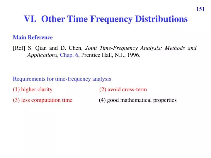
VI. Other Time Frequency Distributions. Main Reference [Ref] S. Qian and D. Chen, Joint Time-Frequency Analysis: Methods and Applications , Chap. 6 , Prentice Hall, N.J., 1996. Requirements for time-frequency analysis: (1) higher clarity (2) avoid cross-term

E N D
VI. Other Time Frequency Distributions Main Reference [Ref] S. Qian and D. Chen, Joint Time-Frequency Analysis: Methods and Applications, Chap. 6, Prentice Hall, N.J., 1996. Requirements for time-frequency analysis: (1) higher clarity (2) avoid cross-term (3) less computation time (4) good mathematical properties
VI-A Cohen’s Class Distribution VI-A-1 Ambiguity Function (1) If
WDF and AF for the signal with only 1 term f t WDF AF
(2) If x1(t) x2(t)
WDF and AF for the signal with 2 terms f auto term |WDF| (t1, f1) cross terms (t , f) t (t2, f2) |AF| cross term auto term (td , fd) auto terms (0, 0) cross term (-td , -fd)
For the ambiguity function The auto term is always near to the origin The cross-term is always far from the origin
VI-A-2 Definition of Cohen’s Class Distribution The Cohen’s Class distribution is a further generalization of the Wigner distribution function where is the ambiguity function (AF). (, ) = 1 WDF where
How does the Cohen’s class distribution avoid the cross term? Chose (, ) low pass function. (, ) 1 for small | |, | | (, ) 0 for large | |, | | [Ref] L. Cohen, “Generalized phase-space distribution functions,” J. Math. Phys., vol. 7, pp. 781-806, 1966. [Ref] L. Cohen, Time-Frequency Analysis, Prentice-Hall, New York, 1995.
VI-A-3 Several Types of Cohen’s Class Distribution Choi-Williams Distribution (One of the Cohen’s class distribution) [Ref] H. Choi and W. J. Williams, “Improved time-frequency representation of multicomponent signals using exponential kernels,” IEEE. Trans. Acoustics, Speech, Signal Processing, vol. 37, no. 6, pp. 862-871, June 1989.
Cone-Shape Distribution (One of the Cohen’s class distribution) [Ref] Y. Zhao, L. E. Atlas, and R. J. Marks, “The use of cone-shape kernels for generalized time-frequency representations of nonstationary signals,” IEEE Trans. Acoustics, Speech, Signal Processing, vol. 38, no. 7, pp. 1084-1091, July 1990.
VI-A-4 Advantages and Disadvantages of Cohen’s Class Distributions The Cohen’s class distribution may avoid the cross term and has higher clarity. However, it requires more computation time and lacks of well mathematical properties. Moreover, there is a tradeoff between the quality of the auto term and the ability of removing the cross terms.
VI-A-5 Implementation for the Cohen’s Class Distribution 簡化法 1:不是所有的 Ax(, ) 的值都需要算出 If for || > B or || > C
簡化法 2:注意, 這個參數和input 及output 都無關 由於 和 input 無關,可事先算出,所以只剩 2 個積分式
VI-B Modified Wigner Distribution Function where X(f) = FT[x(t)] Modified Form I Modified Form II
Modified Form III (Pseudo L-Wigner Distribution) 增加 L可以減少 cross term 的影響 (但是不會完全消除) [Ref] L. J. Stankovic, S. Stankovic, and E. Fakultet, “An analysis of instantaneous frequency representation using time frequency distributions-generalized Wigner distribution,” IEEE Trans. on Signal Processing, pp. 549-552, vol. 43, no. 2, Feb. 1995 P.S.: 感謝2006年修課的林政豪同學
Modified Form IV (Polynomial Wigner Distribution Function) When q = 2 and d1 = d-1 = 0.5, it becomes the original Wigner distribution function. It can avoid the cross term when the order of phase of the exponential function is no larger than q/2 + 1. However, the cross term between two components cannot be removed. [Ref] B. Boashash and P. O’Shea, “Polynomial Wigner-Ville distributions & their relationship to time-varying higher order spectra,” IEEE Trans. Signal Processing, vol. 42, pp. 216–220, Jan. 1994. P.S.: 感謝2011年修課的張一凡同學
VI-C S Transform (Gabor transform 的修正版) closely related to the wavelet transform advantages and disadvantages [Ref] R. G. Stockwell, L. Mansinha, and R. P. Lowe, “Localization of the complex spectrum: the S transform,” IEEE Trans. Signal Processing, vol. 44, no. 4, pp. 998–1001, Apr. 1996.
S transform 和 Gabor transform 相似。 但是 Gaussian window 的寬度會隨著 f而改變 低頻: worse time resolution, better frequency resolution 高頻: better time resolution, worse frequency resolution The result of the S transform (compared with page 82) f-axis t-axis
VI-D Gabor-Wigner Transform [Ref] S. C. Pei and J. J. Ding, “Relations between Gabor transforms and fractional Fourier transforms and their applications for signal processing,” IEEE Trans. Signal Processing, vol. 55, no. 10, pp. 4839-4850, Oct. 2007. Advantages: combine the advantage of the WDF and the Gabor transform advantage of the WDF higher clarity advantage of the Gabor transform no cross-term
(a) (b) (c) (d) (b)、(c) are real
思考: (1) Which type of the Gabor-Wigner transform is better? (2) Can we further generalize the results?
Implementation of the Gabor-Wigner Transform :簡化技巧 (1) When Gx(t, f) 0, 先算 Gx(t, f) Wx(t, f) 只需算 Gx(t, f) 不近似於 0 的地方 (2) When x(t) is real,對 Gabor transform 而言 if x(t) is real, where X(f) = FT[x(t)]
VI-E Generalized Spectrogram [Ref] P. Boggiatto, G. De Donno, and A. Oliaro, “Two window spectrogram and their integrals," Advances and Applications, vol. 205, pp. 251-268, 2009. Generalized spectrogram: Original spectrogram: w1(t) = w2(t) To achieve better clarity, w1(t) can be chosen as a wider window, w2(t) can be chosen as a narrower window.
VI-F Basis Expansion Time-Frequency Analysis 就如同 Fourier series: m(t) = exp(j2fmt), Cosine transform: if g(t) is even, 部分的 Time-Frequency Analysis 也是意圖要將 signal 表示成如下的型態 並且要求在 M固定的情形下, 為最小
(1) Matching Pursuit Hm(t): mth order Hermite function [Ref] S. G. Mallat and Z. Zhang, “Matching pursuits with time-frequency dictionaries,” IEEE Trans. on Signal Processing, vol. 41, no. 12, pp. 3397-3415, Dec. 1993.
(2) Prolate Spheroidal Wave Function (PSWF) Concept: FT: , x, f (, ). energy preservation property (Parseval’s property) finite Fourier transform (fi-FT): space interval: t [T, T], frequency interval: f [, ]
Prolate spheroidal wave functions (PSWFs) are the continuous functions that satisfy: , where . PSWFs are orthogonal and can be sorted according to the values of n,T,’s: 1 > 0,T, > 1,T, > 2,T, > …………. > 0. (All of n,T,’s are real)
During the time interval t [T, T], any function x(t) can be expanded as a linear combination of T,,0(t), T,,1(t), T,,2(t), T,,3(t), ……………. Then it can be shown that the energy ratio of Xfi(f) to x(t) is [Ref] D. Slepian and H. O. Pollak, “Prolate spheroidal wave functions, Fourier analysis and uncertainty-I,” Bell Syst. Tech. J., vol. 40, pp. 43-63, 1961.