Download
1 / 29
290 likes | 445 Views
Learning and Matching of Dynamic Shape Manifolds for Human Action Recognition. Liang Wang and David Suter 2007 IEEE. Outline. Introduction Contribution LPP Activity Classification Results. Introduction.

E N D
Learning and Matching of Dynamic Shape Manifolds for Human Action Recognition Liang Wang and David Suter 2007 IEEE
Outline • Introduction • Contribution • LPP • Activity Classification • Results
Introduction • The silhouettes can be regarded as points in a high-dimensional visual space, and these points may lie on a low-dimensional manifold embedded in the high-dimensional image space.
Introduction • Exploit local preserving projections (LPP) for dimensionality reduction • The associated sequences of dynamic silhouettes are used to learn the activity space using LPP • To match activity trajectories in the low-dimension embedding space, two kinds of motion similarity measures are used.
Contribution • The proposed method has several desirable properties: • Easier to comprehend and implement, without the requirements of explicit feature tracking and complex probabilistic modeling of motion patterns. • Being based on binary silhouette analysis, it naturally avoids some problems arising in most previous methods, e.g., unreliable 2-D or 3-D tracking, expensive and sensitive optical flow. • Obtains good results on a large and challenging database and exhibits considerable robustness.
Methods of Dimensionality Reduction • Curse of dimensionality. • LPP based on linear projective maps that arise by solving a variational problem that optimally preserves the neighborhood structure of the data set.
Brief Introduction to LPP • Constructing the adjacency graph • 該圖的點即是所有的測試資料,而判斷任兩點之間是否有邊相連則有兩種方式,可依需求選擇 • ε-neighborhoods: 若兩點之間的距離小於某個常數ε,則兩點之間有邊相連 • k –nearest neighbors: 若兩點中,有一點在另外一點於整組資料中最相近的K個點中,則兩點之間有邊相連 • Choosing the weights • Eigenmaps
Brief Introduction to LPP • Constructing the adjacency graph • Choosing the weights • 若在第一步驟的圖中兩點之間沒有邊相連,則相關性為0,否則將給定一個相關性,有兩種方式可供選擇,W是一個sparse和對稱矩陣 • More simply: Wij = 1 • Or Heat kernel: Wij = • Eigenmaps
Brief Introduction to LPP • Constructing the adjacency graph • Choosing the weights • Eigenmaps (找出投影矩陣) • 最佳化的投影矩陣保留了locality可以由minimize下面的objective function求出
Brief Introduction to LPP • 依照相關性,找出投影矩陣A • 此時每組aj都獨立作用,所以改為考慮 • 其中a代表某一個投影向量,令 則 D是一個對角矩陣,Dii = L = D-W稱作Laplacian Matrix Y代表所有資料在a這個維度上面的投影
Brief Introduction to LPP • 因為目前僅對轉換後的點之間的相關性作要求,還需要一些轉換後座標上的限制 • 觀察D發現Dii代表與第i點相連的點數有多少,也說明了此點的重要性,所以限制 • 此一限制可讓越重要的點轉換出來的座標值越接近0,亦即將原點設在最密集的區域,此時所求的式子變成 • 最小值出現在 • 經過矩陣的微分運算可得 • 把問題簡化成一個solution of generalized eigenvalue and eigenvector problem.
Brief Introduction to LPP • 另外 因為我們希望 越小越好,所以取a為特徵最小的M個非0特徵向量
Representations of Visual Inputs • The results of transformation is a grayscale image that look similar to the input image. • The distance transform assigns a number that is the distance between the pixel and the nearest nonzero pixel of raw.
Activity Classification • Assume that two action sequences are respectively mapped into A1(L*T1) and A2(L*T2). • L: the reduced dimensionality. • T1 and T2: the durations of these two complete actions respectively. • We select two kinds of distance metrics to measure the motion similarity. • Classifier
Motion Similarity • Similarity-I: Normalized spatiotemporal correlation • The computation usually requires knowing the temporal duration of each one action for such an approximate frame-to-frame matching. • s and b explain time stretch and shifting respectively, T as max(T1,T2). • We wrap each action trajectory matrix into the same temporal duration T by the bicubic interpolation.
Motion Similarity • Similarity-II: Median Hausdorff Distance • A means of determining the resemblance of one point set to another, by examining the fraction of points in one set that lie near points in the other set.
Classifier • Action classification is performed in a nearest neighbour framework • TA: a test action sequence • Ri: the ith reference action sequence • d: similarity measure • Classify the test as the class c that can minimize the similarity distance between test sequence and all reference pattern. • d is the similarity measure d1 or d2 defined above
Results - data processing • To estimate the action cycle of each silhouette. • The object Ot’s self-similarity is computed at time t1 and t2 based on the similarity measure of the absolute correlation. • Bt1 is the bounding box of the object Ot1. • In order to account for tracking error, the minimal S is found by translating over a small search radius r.
Results – results and analysis • Identification mode: • the classifier determines which class a given measurement belongs to in the nearest-neighbor framework
Results – results and analysis • verification mode: • The classifier is asked to verify whether a new measurement really belongs to certain claimed class
Results – results and analysis • Reduced dimension: • Examine the relationship between the reduced dimensions and the recognition rates
Results – results and analysis • Confusion matrix: • For the unsupervised LPP, there exist a few false classifications. To analyze which action are incorrectly classified
Results – robustness test • Corrupted silhouettes by real occlusions:
Results – robustness test • Corrupted silhouettes by real occlusions:
Results – robustness test • Corrupted silhouettes by real occlusions:
Results – robustness test • Other challenging factors: • viewpoints different clothes motion styles
Results - comparisons • Differentdimension reduction methods