Hidden Markov Models

Hidden Markov Models Julia Hirschberg CS4705 CS 4705

POS Tagging using HMMs • A different approach to POS tagging • A special case of Bayesian inference • Related to the “noisy channel” model used in MT, ASR and other applications 3/12/2014 2

POS Tagging as a Sequence ID Task • Given a sentence (a sequence of words, or observations) • Secretariat is expected to race tomorrow • What is the best sequence of tags which corresponds to this sequence of observations? • Bayesian approach: • Consider all possible sequences of tags • Choose the tag sequence t1…tn which is most probable given the observation sequence of words w1…wn 3/12/2014 3

Out of all sequences of n tags t1…tn want the single tag sequence such that P(t1…tn|w1…wn) is highest • I.e. find our best estimate of the sequence that maximizes P(t1…tn|w1…wn) • How do we do this? • Use Bayes rule to transform P(t1…tn|w1…wn) into a set of other probabilities that are easier to compute 3/12/2014 4

Bayes Rule • Bayes Rule • Rewrite • Substitute 3/12/2014 5

Drop denominator since is the same for all we consider • So….

Likelihoods, Priors, and Simplifying Assumptions • A1:P(w) depends only on its own POS • A2:P(t) depends only on P(t-1) n

Simplified Equation • Now we have two probabilities to calculate: • Probability of a word occurring given its tag • Probability of a tag occurring given a previous tag • We can calculate each of these from a POS-tagged corpus

Tag Transition Probabilities P(ti|ti-1) • Determiners likely to precede adjs and nouns but unlikely to follow adjs • The/DT red/JJ hat/NN;*Red/JJ the/DT hat/NN • So we expect P(NN|DT) and P(JJ|DT) to be high but P(DT|JJ) to be low • Compute P(NN|DT) by counting in a tagged corpus:

Word Likelihood Probabilities P(wi|ti) • VBZ (3sg pres verb) likely to be is • Compute P(is|VBZ) by counting in a tagged corpus: 3/12/2014 10

Some Data on race • Secretariat/NNP is/VBZ expected/VBN to/TO race/VB tomorrow/NR • People/NNS continue/VB to/TO inquire/VB the/DT reason/NN for/IN the/DTrace/NN for/IN outer/JJ space/NN • How do we pick the right tag for race in new data? 3/12/2014 11

Disambiguating to race tomorrow 3/12/2014 12

Markov Chains • Markov Chains • Have transition probabilities like P(ti|ti-1) • A special case of weighted FSTs (FSTs which have probabilities or weights on the arcs) • Can only represent unambiguous phenomena 3/12/2014 14

A Weather Example: cold, hot, hot 3/12/2014 15

Weather Markov Chain • What is the probability of 4 consecutive rainy days? • Sequence is rainy-rainy-rainy-rainy • I.e., state sequence is 3-3-3-3 • P(3,3,3,3) = • 1a33a33a33a33 = 0.2 x (0.6)3 = 0.0432 3/12/2014 16

Markov Chain Defined • A set of states Q = q1, q2…qN • Transition probabilities • A set of probabilities A = a01a02…an1…ann. • Each aij represents the probability of transitioning from state i to state j • The set of these is the transition probability matrix A • Distinguished start and end states q0,qF 3/12/2014 17

Can have special initial probability vector  instead of start state • An initial distribution over probability of start states • Must sum to 1 18 3/12/2014

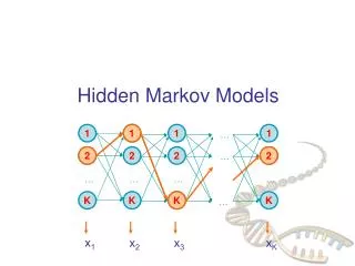
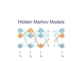
Hidden Markov Models • Markov Chains are useful for representing problems in which • Observable events • Sequences to be labeled are unambiguous • Problems like POS tagging are neither • HMMs are useful for computing events we cannot directly observe in the world, using other events we can observe • Unobservable (Hidden): e.g., POS tags • Observable: e.g., words • We have to learn the relationships

Hidden Markov Models • A set of states Q = q1, q2…qN • Transition probabilities • Transition probability matrix A = {aij} • Observations O= o1, o2…oN; • Each a symbol from a vocabulary V = {v1,v2,…vV} • Observation likelihoods or emission probabilities • Output probability matrix B={bi(ot)}

Special initial probability vector  • A set of legal accepting states 3/12/2014 21

First-Order HMM Assumptions • Markov assumption: probability of a state depends only on the state that precedes it • This is the same Markov assumption we made when we decided to represent sentence probabilities as the product of bigram probabilities • Output-independence assumption: probability of an output observation depends only on the state that produced the observation 3/12/2014 22

Weather Again 3/12/2014 23

Weather and Ice Cream • You are a climatologist in the year 2799 studying global warming • You can’t find any records of the weather in Baltimore for summer of 2007 • But you find JE’s diary • Which lists how many ice-creams J ate every day that summer • Your job: Determine (hidden) sequence of weather states that `led to’ J’s (observed) ice cream behavior 3/12/2014 24

Weather/Ice Cream HMM • Hidden States: {Hot,Cold} • Transition probabilities (A Matrix) between H and C • Observations: {1,2,3} # of ice creams eaten per day • Goal: Learn observation likelihoods between observations and weather states (Output Matrix B) by training HMM on aligned input streams from a training corpus • Result: trained HMM for weather prediction given ice cream information alone

Ice Cream/Weather HMM 3/12/2014 26

HMM Configurations Ergodic = fully-connected Bakis = left-to-right

What can HMMs Do? • Likelihood: Given an HMM λ = (A,B) and an observation sequence O, determine the likelihood P(O, λ): Given # ice creams, what is the weather? • Decoding: Given an observation sequence O and an HMM λ = (A,B), discover the best hidden state sequence Q: Given seq of ice creams, what was the most likely weather on those days? • Learning: Given an observation sequence O and the set of states in the HMM, learn the HMM parameters A and B 3/12/2014 28

Likelihood: The Forward Algorithm • Likelihood: Given an HMM λ = (A,B) and an observation sequence O, determine the likelihood P(O, λ) • E.g. what is the probability of an ice-cream sequence 3 – 1 – 3 given 3/12/2014 29

Compute the joint probability of 3 – 1 – 3 by summing over all the possible {H,C} weather sequences – since weather is hidden • Forward Algorithm: • Dynamic Programming algorithm, stores table of intermediate values so it need not recompute them • Computes P(O) by summing over probabilities of all hidden state paths that could generate the observation sequence 3 -- 1 – 3:

The previous forward path probability, • The transition probability from the previous state to the current state • The state observation likelihood of the observation ot given the current state j

Decoding: The Viterbi Algorithm • Decoding: Given an observation sequence O and an HMM λ = (A,B), discover the best hidden state sequence of weather states in Q • E.g., Given the observations 3 – 1 – 1 and an HMM, what is the best (most probable) hidden weather sequence of {H,C} • Viterbi algorithm • Dynamic programming algorithm • Uses a dynamic programming trellis to store probabilities that the HMM is in state j after seeing the first t observations, for all states j 3/12/2014 32

Value in each cell computed by taking MAX over all paths leading to this cell – i.e. best path • Extension of a path from state i at time t-1 is computed by multiplying: • Most probable path is the max over all possible previous state sequences • Like Forward Algorithm, but it takes the max over previous path probabilities rather than sum

HMM Training: The Forward-Backward (Baum-Welch) Algorithm • Learning: Given an observation sequence O and the set of states in the HMM, learn the HMM parameters A (transition) and B (emission) • Input: unlabeled seq of observations O and vocabulary of possible hidden states Q • E.g. for ice-cream weather: • Observations = {1,3,2,1,3,3,…} • Hidden states = {H,C,C,C,H,C,….}

Intuitions • Iteratively re-estimate counts, starting from an initialization for A and B probabilities, e.g. all equi-probable • Estimate new probabilities by computing forward probability for an observation, dividing prob. mass among all paths contributing to it, and computing the backward probability from the same state • Details: left as an exercise to the Reader

Very Important • Check errata for Chapter 6 – there are some important errors in equations • Please use clic.cs.columbia.edu, not cluster.cs.columbia.edu for HW

Summary • HMMs are a major tool for relating observed sequences to hidden information that explains or predicts the observations • Forward, Viterbi, and Forward-Backward Algorithms are used for computing likelihoods, decoding, and training HMMs • Next week: Sameer Maskey will discuss Maximum Entropy Models and other Machine Learning approaches to NLP tasks • These will be very useful in HW2

Hidden Markov Models