Download
1 / 47
470 likes | 689 Views
Spatial and Temporal Data Mining. Clustering I. Vasileios Megalooikonomou. (based on notes by Jiawei Han and Micheline Kamber). Agenda. What is Cluster Analysis? Types of Data in Cluster Analysis A Categorization of Major Clustering Methods Partitioning Methods Hierarchical Methods

E N D
Spatial and Temporal Data Mining Clustering I Vasileios Megalooikonomou (based on notes by Jiawei Han and Micheline Kamber)
Agenda • What is Cluster Analysis? • Types of Data in Cluster Analysis • A Categorization of Major Clustering Methods • Partitioning Methods • Hierarchical Methods • Density-Based Methods • Grid-Based Methods • Model-Based Clustering Methods • Outlier Analysis • Summary
Typical Applications of Clustering • Pattern Recognition • Spatial Data Analysis • create thematic maps in GIS by clustering feature spaces • detect spatial clusters and explain them in spatial data mining • e.g., land use, city planning, earth-quake studies • Image Processing • Economic Science (especially market research) – e.g., marketing, insurance • WWW • Document classification • Cluster Weblog data to discover groups of similar access patterns
What Is Good Clustering? • A good clustering method will produce high quality clusters with • high intra-class similarity • low inter-class similarity • The quality of a clustering result depends on both the similarity measure used by the method and its implementation. • The quality of a clustering method is also measured by its ability to discover some or all of the hidden patterns.
Requirements of Clustering in Data Mining • Scalability • Ability to deal with different types of attributes • Discovery of clusters with arbitrary shape (not just spherical clusters) • Minimal requirements for domain knowledge to determine input parameters (such as # of clusters) • Able to deal with noise and outliers • Insensitive to order of input records • Incremental clustering • High dimensionality (especially very sparse and highly skewed data) • Incorporation of user-specified constraints • Interpretability and usability (close to semantics)
Agenda • What is Cluster Analysis? • Types of Data in Cluster Analysis • A Categorization of Major Clustering Methods • Partitioning Methods • Hierarchical Methods • Density-Based Methods • Grid-Based Methods • Model-Based Clustering Methods • Outlier Analysis • Summary
Types of Data and Data Structures • Data matrix • (two modes) n objects, p variables • Dissimilarity matrix • (one mode) between all pairs of n objects
Measure the Quality of Clustering • Dissimilarity/Similarity metric: Similarity is expressed in terms of a distance function, which is typically metric: d(i, j) • There is a separate “quality” function that measures the “goodness” of a cluster. • The definitions of distance functions are usually very different for interval-scaled, boolean, categorical, ordinal and ratio variables. • Weights should be associated with different variables based on applications and data semantics. • Hard to define “similar enough” or “good enough” • highly subjective.
Interval-valued variables • Continuous measurements of a roughly linear scale (e.g., weight, height, temperature, etc) • Standardize data (to avoid dependence on the measurement units) • Calculate the mean absolute deviation of a variable f with n measurements: where • Calculate the standardized measurement (z-score) • Using mean absolute deviation is more robust (to outliers) than using standard deviation
Similarity and Dissimilarity Between Objects • Distances are normally used to measure the similarity or dissimilarity between two data objects • Some popular ones include: Minkowski distance: where i = (xi1, xi2, …, xip) and j = (xj1, xj2, …, xjp) are two p-dimensional data objects, and q is a positive integer • If q = 1, d is Manhattan distance
Similarity and Dissimilarity Between Objects • If q = 2, d is Euclidean distance: • Properties • d(i,j) 0 • d(i,i)= 0 • d(i,j)= d(j,i), symmetry • d(i,j) d(i,k)+ d(k,j), triangular inequality • Also one can use weighted distance, parametric Pearson product moment correlation, or other dissimilarity measures.
Binary Variables Object j • A contingency table for binary data • Simple matching coefficient (invariant similarity, if the binary variable is symmetric (both states same weight)): • Jaccard coefficient (noninvariant similarity, if the binary variable is asymmetric (states not equally important e.g., outcomes of a disease test)): Object i
Dissimilarity between Binary Variables • Example • gender is a symmetric attribute • the remaining attributes are asymmetric binary • let the values Y and P be set to 1, and the value N be set to 0
Nominal Variables • A generalization of the binary variable in that it can take more than 2 states, e.g., red, yellow, blue, green • Method 1: Simple matching • m: # of matches (# of variables for which i and j are in the same state), p: total # of variables • Method 2: use a large number of binary variables • creating a new binary variable for each of the M nominal states
Ordinal Variables • An ordinal variable can be discrete or continuous • Resembles nominal var but order is important, e.g., rank • Can be treated like interval-scaled • replace xif by their rank where ordinal variable f has Mf states and xif is the value of f for the i-th object • map the range of each variable onto [0, 1] by replacing the rank of the i-th object in the f-th variable by • compute the dissimilarity using methods for interval-scaled variables
Ratio-Scaled Variables • Ratio-scaled variable: a positive measurement on a nonlinear scale, approximately at exponential scale, such as AeBt or Ae-Bt where A and B are positive constants (e.g., decay of radioactive elements) • Methods: • treat them like interval-scaled variables — not a good choice! (why?) • apply logarithmic transformation yif = log(xif) and treat them as interval-valued • treat them as continuous ordinal data and treat their rank as interval-scaled.
Variables of Mixed Types • A database may contain all the six types of variables • symmetric binary, asymmetric binary, nominal, ordinal, interval and ratio. • One may use a weighted formula to combine their effects. • f is binary or nominal: dij(f) = 0 if xif = xjf , or dij(f) = 1 otherwise. • f is interval-based: use the normalized distance • f is ordinal or ratio-scaled • compute ranks rif and • and treat zif as interval-scaled
Agenda • What is Cluster Analysis? • Types of Data in Cluster Analysis • A Categorization of Major Clustering Methods • Partitioning Methods • Hierarchical Methods • Density-Based Methods • Grid-Based Methods • Model-Based Clustering Methods • Outlier Analysis • Summary
Clustering Approaches • Partitioning algorithms: Construct various partitions and then evaluate them by some criterion (k-means, k-medoids) • Hierarchical algorithms: Create a hierarchical decomposition (agglomerative or divisive) of the set of data (or objects) using some criterion (CURE, Chameleon, BIRCH) • Density-based: based on connectivity and density functions – grow a cluster as long as density in the neighborhood exceeds a threshold (DBSCAN, CLIQUE) • Grid-based: based on a multiple-level grid structure (i.e., quantized space) (STING, CLIQUE) • Model-based: A model is hypothesized for each of the clusters and the idea is to find the best fit of the data to the given model (EM)
Agenda • What is Cluster Analysis? • Types of Data in Cluster Analysis • A Categorization of Major Clustering Methods • Partitioning Methods • Hierarchical Methods • Density-Based Methods • Grid-Based Methods • Model-Based Clustering Methods • Outlier Analysis • Summary
Partitioning Algorithms: Basic Concept • Partitioning method: Construct a partition of a database D of n objects into a set of k clusters • Given a k, find a partition of k clusters that optimizes the chosen partitioning criterion • Global optimal: exhaustively enumerate all partitions • Heuristic methods: k-means and k-medoids algorithms • k-means (MacQueen’67): Each cluster is represented by the center of the cluster • k-medoids or PAM (Partition around medoids) (Kaufman & Rousseeuw’87): Each cluster is represented by one of the objects in the cluster
The K-Means Clustering Method • Given k, the k-means algorithm is implemented in 4 steps: 1. Partition objects into k nonempty subsets • Compute seed points as the centroids of the clusters of the current partition. The centroid is the center (mean point) of the cluster. • Assign each object to the cluster with the nearest seed point. • Go back to Step 2, stop when no more new assignment (or fractional drop of SSE or MSE is less than a threshold).
The K-Means Clustering Method • Example
Comments on the K-Means Method • Strengths • Relatively efficient: O(tkn), where n is # objects, k is # clusters, and t is # iterations. Normally, k, t << n. • Often terminates at a local optimum. The global optimum may be found using techniques such as: deterministic annealing and genetic algorithms • Weaknesses • Applicable only when mean is defined, then what about categorical data? • Need to specify k, the number of clusters, in advance • Unable to handle noisy data and outliers • Not suitable to discover clusters with non-convex shapes
Variations of the K-Means Method • A few variants of the k-means which differ in • Selection of the initial k means • Dissimilarity calculations • Strategies to calculate cluster means • Handling categorical data: k-modes (Huang’98) • Replacing means of clusters with modes • Using new dissimilarity measures to deal with categorical objects • Using a frequency-based method to update modes of clusters • A mixture of categorical and numerical data: k-prototype method
The K-MedoidsClustering Method • Find representative (i.e., the most centrally located) objects, called medoids, in clusters • PAM (Partitioning Around Medoids, 1987) • starts from an initial set of medoids and iteratively replaces one of the medoids by one of the non-medoids if it improves the total distance of the resulting clustering • PAM works effectively for small data sets, but does not scale well for large data sets • More robust than k-means • Complexity: O(k(n-k)2) for n objects and k clusters • CLARA (Kaufmann & Rousseeuw, 1990): Uses multiple samples • CLARANS (Ng & Han, 1994): Randomized sampling • Focusing + spatial data structure (Ester et al., 1995)
PAM (Partitioning Around Medoids) (1987) • PAM (Kaufman and Rousseeuw, 1987), built in Splus • Use real object to represent the cluster • Select k representative objects arbitrarily • For each pair of non-selected object h and selected object i, calculate the total swapping cost Tcih • For each pair of i and h, • If TCih < 0, i is replaced by h • Then assign each non-selected object to the most similar representative object 4. repeat steps 2-3 until there is no change
j t t j h i h i h j i i h j t t PAM Clustering:Total swapping cost TCih=jCjih
CLARA (Clustering Large Applications) (1990) • CLARA (Kaufmann and Rousseeuw in 1990)(O(ks2 + k(n-k))) • Built in statistical analysis packages, such as S+ • It draws multiple samples of the data set, applies PAM on each sample, and gives the best clustering as the output • Strength:deals with larger data sets than PAM • Weakness: • efficiency depends on the sample size and … • the sample: A good clustering based on samples will not necessarily represent a good clustering of the whole data set if the sample is biased
CLARANS (“Randomized” CLARA) (1994) • CLARANS (A Clustering Algorithm based on Randomized Search) (Ng and Han’94) (O(n2)) • CLARANS draws a sample of neighbors dynamically • The clustering process can be presented as searching a graph where every node is a potential solution, that is, a set of k medoids • If the local optimum is found, CLARANS starts with new randomly selected node in search for a new local optimum • It is more efficient and scalable than both PAM and CLARA • Focusing techniques and spatial access structures may further improve its performance (Ester et al.’95)
Agenda • What is Cluster Analysis? • Types of Data in Cluster Analysis • A Categorization of Major Clustering Methods • Partitioning Methods • Hierarchical Methods • Density-Based Methods • Grid-Based Methods • Model-Based Clustering Methods • Outlier Analysis • Summary
Step 0 Step 1 Step 2 Step 3 Step 4 agglomerative (AGNES) a a b b a b c d e c c d e d d e e divisive (DIANA) Step 3 Step 2 Step 1 Step 0 Step 4 Hierarchical Clustering • Use distance matrix as clustering criteria. This method does not require the number of clusters k as an input, but needs a termination condition
AGNES (Agglomerative Nesting) • Introduced in Kaufmann and Rousseeuw (1990) • Implemented in statistical analysis packages, e.g., Splus • Use the Single-Link method and the dissimilarity matrix: • each cluster is represented by all of its objects and the similarity between clusters is measured by the similarity of the closest pair of data points belonging to different clusters • Merge nodes that have the least dissimilarity • Go on in a non-descending fashion • Eventually all nodes belong to the same cluster
A Dendrogram Shows How the Clusters are Merged Hierarchically • Decompose data objects into a several levels of nested partitioning (tree of clusters), called a dendrogram. • A clustering of the data objects is obtained by cutting the dendrogram at the desired level, then each connected component forms a cluster.
DIANA (Divisive Analysis) • Introduced in Kaufmann and Rousseeuw (1990) • Implemented in statistical analysis packages, e.g., Splus • Inverse order of AGNES • Eventually each node forms a cluster on its own
More on Hierarchical Clustering Methods • Major weakness of agglomerative clustering methods • do not scale well: time complexity of at least O(n2), where n is the number of total objects • can never undo (backtrack) what was done previously • Integration of hierarchical with distance-based clustering • BIRCH (1996): uses CF-tree (clustering feature tree) and incrementally adjusts the quality of sub-clusters • CURE (1998): selects well-scattered (representative) points from the cluster and then shrinks them towards the center of the cluster by a specified fraction • CHAMELEON (1999): hierarchical clustering using dynamic modeling
BIRCH (1996) • Birch: Balanced Iterative Reducing and Clustering using Hierarchies, by Zhang, Ramakrishnan, Livny (SIGMOD’96) • Incrementally construct a CF (Clustering Feature) tree, a hierarchical data structure for multiphase clustering • Phase 1: scan DB to build an initial in-memory CF tree (a multi-level compression of the data that tries to preserve the inherent clustering structure of the data) • Phase 2: use an arbitrary clustering algorithm to cluster the leaf nodes of the CF-tree • Scales linearly: finds a good clustering with a single scan and improves the quality with a few additional scans • Weakness: handles only numeric data, and sensitive to the order of the data record.
Clustering Feature:CF = (N, LS, SS) N: Number of data points LS: Ni=1Xi SS: Ni=1Xi2 Clustering features are additive Clustering Feature Vector CF = (5, (16,30),(54,190)) (3,4) (2,6) (4,5) (4,7) (3,8)
B: Branching factor: max # children per nonleaf node L: Threshold: max diameter of subclusters at leaf nodes CF1 CF2 CF3 CF6 child1 child2 child3 child6 CF Tree Root B = 7 L = 6 Non-leaf node CF1 CF2 CF3 CF5 child1 child2 child3 child5 Leaf node Leaf node prev CF1 CF2 CF6 next prev CF1 CF2 CF4 next
CURE (Clustering Using REpresentatives ) • CURE: proposed by Guha, Rastogi & Shim, 1998 (O(n)) • Stops the creation of a cluster hierarchy if a level consists of k clusters • Uses multiple representative points to evaluate the distance between clusters • Adjusts well to arbitrary shaped clusters and avoids single-link effect
Drawbacks of Distance-Based Method • Drawbacks of square-error based clustering method • Consider only one point as representative of a cluster • Good only for convex shaped, similar size and density, and if k can be reasonably estimated
Cure: The Algorithm • Draw random sample s. • Partition sample to p partitions with size s/p • Partially cluster partitions into s/pq clusters • Eliminate outliers • By random sampling • If a cluster grows too slow, eliminate it. • Cluster partial clusters. • Label data in disk
y y y x y y x x Data Partitioning and Clustering • s/pq = 5 • s = 50 • p = 2 • s/p = 25 x x
y y x x Cure: Shrinking Representative Points • Shrink the multiple representative points towards the gravity center by a fraction of . • Multiple representatives capture the shape of the cluster
Clustering Categorical Data: ROCK • ROCK: Robust Clustering using linKs,by S. Guha, R. Rastogi, K. Shim (ICDE’99). • Use links to measure similarity/proximity (# points from different clusters who have neighbors in common) -> # of links of two points = # common neighbors • Not distance based • Hierarchical clustering • Computational complexity: • Basic ideas: • Similarity function and neighbors: Let T1 = {1,2,3}, T2={3,4,5}
CHAMELEON • CHAMELEON: hierarchical clustering using dynamic modeling, by G. Karypis, E.H. Han and V. Kumar’99 (O(n2)) • Measures the similarity based on a dynamic model • Two clusters are merged only if the interconnectivityand closeness (proximity) between two clusters are high relative to the internal interconnectivity of the clusters and closeness of items within the clusters • A two phase algorithm • 1. Use a graph partitioning algorithm: cluster objects into a large number of relatively small sub-clusters • 2. Use an agglomerative hierarchical clustering algorithm: find the genuine clusters by repeatedly combining these sub-clusters
Overall Framework of CHAMELEON Construct Sparse Graph Partition the Graph Data Set Merge Partition Final Clusters It uses a k-nearest neighbor approach to construct the sparse graph: Each vertex represents an object, an edge exists between two vertices if one object is among the k-most similar objects of the other