Download
1 / 29
290 likes | 483 Views
COS Training Series IV: COS Post-observation. M.E. Kaiser P. E. Hodge 28 February 2008. COS Spectrograph (Colorado, BASG). COS Pipeline Verification. STScI : Mary Elizabeth Kaiser Phil Hodge Tony Keyes Tom Ake Cristina Oliveira Dave Sahnow Brittany Shaw Alessandra Aloisi Rosa Diaz

E N D
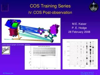
COS Training SeriesIV: COS Post-observation M.E. Kaiser P. E. Hodge 28 February 2008 COS Spectrograph (Colorado, BASG)
COS Pipeline Verification • STScI : • Mary Elizabeth Kaiser • Phil Hodge • Tony Keyes • Tom Ake • Cristina Oliveira • Dave Sahnow • Brittany Shaw • Alessandra Aloisi • Rosa Diaz • Charles Proffitt • Colorado: • Jim Green • Stephane Beland • Steve Penton • Eric Burgh • Cyndi Froning • Steve Osterman • Eric Wilkinson
COS Pipeline • Outline • Pipeline Description • Python • Data Formats and File Structure • Calibration Reference Files & Tables • Reduced Data Products, Formats, etc. • Cumulative Image & Pulse Height Maps • Headers and Keywords
CALCOS Foundation CALCOS: Python program to calibrate COS FUV & NUV TIME_TAG event lists & ACCUM images, producing a wavelength & flux calibrated spectrum. • CALCOS data requirements specified by AV03(COS Calibration Requirements & Procedures) • Outlines final data products for COS observations • Specifies the pre-flight calibration requirements • Specifies the reference files required • Specifies the calibration steps required to obtain the COS data product Reminder:
CALCOS Products • TIME-TAG data: • Raw events table: time, x, y, pulse height amplitude (FUV) • Produce corrected events table: time, corrected x, corrected y, weight, dq, pha • Produce calibrated ACCUM image from corrected event list • ACCUM data: • Produce calibrated ACCUM image from raw ACCUM image • Produce flux-calibrated 1-D spectrum (wavelength calibrated) • Combine FP-POS or REPEATOBS spectra • 2-d data: FITS images • - single imset consisting of science, error, & data quality images • 1-d data and TIME-TAG lists: FITS tables • - extracted spectra contain fluxes, wavelengths, errors, data quality, and other related quantities (e.g. background)
Input Files and Products • CALCOS files • Science spectrum (suffix designates detector) • “_a” (or “_b” ): FUV detector segment A (or B); NUV: no “_” • Pulse-height histogram if FUV ACCUM (A and B) • Target-acquisition image • Support file (contains engineering information) • Association file controls calibration processing (science exposures, wavecals) Primary TIME-TAG file products:“rawtag” (raw photon list), “corrtag” (corrected photon list), “flt” (2-D corrected count-rate image), “x1d” (1-D flux-calibrated extracted spectrum). Primary ACCUM file products:“rawimage”(raw image),“flt”,“x1d” 1-D spectrum for each FP-split location or repeatobs exposure; Sum of 1-D spectra All associated data (e.g., wavecals, FP-POS components, REPEATOBS, PHA) use separate files (unlike STIS) & are linked via an association table.
What is Python & Why should we use it? CALCOS is Written in Python Python is an Open Source, freely available “scripting” language for astronomy data reduct’n & analysis • Extremely productive (Many powerful libraries available) • Easy to learn and read & well-documented. • Available on just about any computing platform. Portable with robust implementation • Wide user and developer base • Supports both procedural and object-oriented coding. • Unlike Tcl or Perl, scales well to larger programming projects • Extendable with C, C++, or Fortran. • The Science Software Group successfully developed a new Command Language for IRAF using Python. • Programs more easily written, tested, and modified than C programs because of Python’s interpreted, dynamic and concise nature • Programs easier to adapt to unanticipated cal requirements than C programs. • Better at bookkeeping and set-up than C • Easier to diagnose Python errors than C errors (esp. memory and pointer errors).
CALCOS Overview Reference Files ref_flat.fits flat field image ref_geo.fits geom distort’n file ref_dead.fits livetime factr table ref_bpix.fits dqi table ref_brf.fits baseline (stim loc) table ref_pha.fits pulse height table ref_1dx.fits spectrum loc table ref_lamp.fits template spectrm tbl ref_phot.fits sensitivity ref table ref_dsp.fits dspn relation poly tbl ref_wcp.fits wave params table • User supplies association table name • Read and interpret association table: • get a list of the input files • open one input file to get header keywords: • identify calibration steps to perform • obtain list of reference file names • verify that all required files are present • Calibrate: • Process associated wavecals • determine wavecal offset from ref wavecal • calibrate each input science file • Average the individual FP-split or repeatobs • COS ASSOCIATIONS: will generally follow NICMOS design • - associated obs are in separate datasets linked via an association table • Each spectroscop sci expos will have at least 1 wavecal assoc wavecals may be shared by diff sci exps • Only formal associat’ns in pipeline process & HAD: science/wavecal groupings, FP-POSs, & REPEATOBS
Outline of Calibration Steps TIME-TAG data Copy input data into output array Add pseudo-random number to each X and Y position (FUV only) Thermal correction (FUV only) Geometric correction (FUV only) Flat field correction Livetime correction Data quality assignment Filter by pulse height (FUV only) Filter by time Orbital & heliocentric Doppler corrections Create 2-D ACCUM images
Outline of Calibration Steps (cont.) ACCUM data Verify good pulse-height distribution (FUV only) Find stim pulses and compute thermal distortion coefficients (FUV only) Convert ACCUM to temporary coordinate list (FUV only) Add pseudo-random number to each X and Y position (FUV only) Thermal correction (FUV only) Geometric correction (FUV only) Data quality assignment Compute orbital and heliocentric Doppler shifts Create 2-D temporary count rate ACCUM image Convolve flat field with Doppler shift and divide into count rate image Livetime correction Create 2-D effective count rate image
Outline of Calibration Steps (cont.) Steps common to TIME-TAG and ACCUM Extract 1-D spectrum: Compute net count rate Compute error estimate Compute maximum and average data quality Compute wavelengths Compute flux from count rate Combine FP-split or repeatobs
Running CALCOS: An Example Input FUV spectrum: - source: external Pt/Ne lamp - exposure sequence: 3 FP-POS positions - tagflash exposures through WCA using internal Pt/Ne lamp • Running CALCOS (2 options) • Run calcos.py • from the UNIX command line • Run from Pyraf • (Python w/ IRAF imported) • pyraf • import calcos • stsdas • calcos.calcos (“file.fits”) Tagflash Wavecal Exposure: Internal Pt/Ne lamp (WCA aperture) Science Exposure: External Pt/Ne lamp (PSA aperture)
The Details: Thermal Correction • Electronic stim pulse signals are used to correct the FUV XDL data for thermal drift (The x & y positions of detected photon events are obtained from analog electronics --> susceptible to thermal changes.) • Reference Stim positions used to correct the data to the reference frame • Must be done at the outset before any reference files are applied • NUV MAMA has physical pixels. No stim pulse capability exists or required. 2 stim pulses for each detector Segment, located at the lower left & upper right m Thermal correction done after screening for bursts (outliers in bkg_counts) m
The Details: Geometric Correction • Corrects for optical distortions at the detector image • FUV geometric correction reference file has been delivered by IDT • dx is multiplied by 10 in the geometric distortion map below • for segments A and B to illustrate the distortion characteristics • NUV geometric correction need under evaluation by IDT - effect is small
The Details: Flat Field Correction • Corrects for pixel-pixel variations • FUV flat field under evaluation - in-flight validation planned Top panel: flat field taken pre-TV no grid wires Middle panel: 2003 TV flat field note grid wires Lower panel: same as middle panel but with zoomed y-axis note blemish Grid wires: A negatively charged, primarily vertical grid that increases detector efficiency by inhibiting electrons from scattering out of the MCP pores.
The Details: Flat Field Correction • Corrects for pixel-pixel variations • NUV flat field delivered by IDT zoomed region - note hex structure Full flat field
The Details: Data Quality Assignment • Identifies detector regions of less than optimal performance • Detector dead-zones, hot spots, grid wire shadows, blemishes • Data drop-outs • Note location & • flux level depression for: • grid wire shadows • dead spots • blemishes
The Result FUV spectrum: source: external Pt/Ne lamp exposure sequence: 3 FP-POS positions (PSA aperture) tagflash exposures through WCA aperture using internal Pt/Ne lamp
Lifetime Charge Extraction Detector lifetime is a function of the charge extracted. A cumulative signal image of the FUV & NUV detectors will be maintained to monitor the extracted charge. FUV detector has 5 default positions to mitigate effects of charge extraction (gain sag). (non-concurrent) FUSE cumulative signal image Left: Lyman Beta region Right: Background region Light stripes are grid wire shadows
FUV Pulse Height Maps • The Pulse Height of the electron cloud can be used to • discriminate between science and spurious sources • monitor the lifetime of the microchannel plate (MCP) - • identify regions with large charge extractions (gain sag) Red histogram: Gain sag of the FUSE detector is shown for the Lyman Beta region - which has had large charge extraction due to both airglow and science targets. Black histrogram: Background region with minimal gain sag due to charge extraction.
Data File Naming Conventions • Product Suffix Type Contents • --------------------------------------------------------------------------------------------------------------- • Uncalibrated _rawimage image Raw ACCUM counts image • _rawtag table Raw TIME-TAG event list • _asn table Association file • _trl table Trailer file • _jit table • _jif image • _pha table Pulse-height (FUV ACCUM only) • --------------------------------------------------------------------------------------------------------------- • Calibrated_corrtag table Calibrated TIME-TAG event list • _flt image Flat-fielded, corrected counts • _fltsum image Summed flat-fielded corrected-counts • _x1d table 1-D extracted spectra • _x1dsum table Combined 1-D extracted spectrum • _trl table Trailer file (output) • _spt image Support file (header) • -------------------------------------------------------------------------------------------------------------- • Wavecal expos produce same calibrated files as science, except no flux calibration applied to the _x1* files. Dark, flat, & image exposures produce no _x1* files. Acquisition exposures produce no calibrated products.
COS Configuration Keywords Keyword: some possible values OBSTYPE: SPECTROSCOPIC, IMAGING OBSMODE: ACCUM, TIME-TAG EXPTYPE:ACQ,PEAKUP/XDISP, PEAKUP/DISP, SCI,WAVE,FLAT, DARK,PHA DETECTOR: FUV , NUV SEGMENT: FUVA, FUVB OPT_ELEM:G130M, G160M, G185M, G225M, G285M, G140L,G230L, MIRRORA, MIRRORB CENWAVE:1298, 1309, 1320, etc. APERTURE :PSA, BOA, WCA, FCA (Indicates a COS unique keyword or value)
Keyword specification keyword name default value possible values units datatype short comment for header long description header position DADS table keyword source • The following information is being generated by STScI Science Instrument team and DST for all COS specific keywords.
Association Table Column names MEMNAME, MEMTYPE, MEMPRSNT MEMNAME is the rootname for a file or set of files MEMTYPE distinguishes science from wavecal, and exposure from product MEMPRSNT = true implies that input files with the specified rootname exist
COS Associations Only associations required for data processing will be constructed by TRANS There will be 1 product, and only 1 product, for each association. COS associations will consist of FP-split (always 4) or repeat obs. exposures Wavecals Wavecals executed after each grating, central wavelength, mirror, or aperture change; and at least once each orbit. Wavecals can be shared between associations An association table will contain all information about associated dataset Observations will complete Generic Conversion as individual exposures, be held by a Data Collector until all member exposures are present, and the product will be created by CALCOS.
NUV Science Data Format NUV MAMA PtNe Wavecal External Science C B A C B A