Download
1 / 42
420 likes | 577 Views
Stochastic Volatility Models The Nord Pool Energy Market by Per Bjarte Solibakke Department of Economics, Molde University College. Stochastic Volatility: Origins and Overview.

E N D
Stochastic Volatility Models The Nord Pool Energy Market by Per BjarteSolibakke Department of Economics, Molde University College Trondheim, 29-30th June 2011
Stochastic Volatility: Origins and Overview Stochastic Volatility (SV) models are used to capture the impact of time-varying volatility on financial markets and decision making (endemic in markets) . The success of SV models is multidisciplinary: financial economics, probability theory and econometrics are blended to produce methods that aid our understanding of option pricing, efficient portfolio allocation and accurate risk assessment and management. Heterogeneity has implications for the theory and practice of economics and econometrics. Heterogeneity for asset pricing theory means higher rewards are required as an asset is exposed to more systematic risk. SV models bring us closer to reality, allowing us to make better decisions, inspire new theory and improve model building. Page: 2
Stochastic Volatility: Origins and Overview The SV approach indirectly specifies the predictive distribution of returns via the structure of the scientific model (need numerical computations in most cases). The advantage is that it is more convenient and perhaps more natural to model the volatility as having its own stochastic process. The disadvantage is that the likelihood function is not directly available. From the late 1990s the SV models have taken centre stage in the econometric analysis of volatility forecasting using high-frequency data based on realized volatility (RV) and related concepts. This is mainly due to the fact that the econometric analysis of realized volatility is tied to continuous time processes. The close connection between SV and RV models allows econometricians to harness the enriched information set available through high frequency data to improve, by an order of magnitude, the accuracy of their volatility forecasts. Page: 3
Stochastic Volatility: Origins and Overview The central intuition in the SV literature is that asset returns are well approximated by a mixture distribution where the mixture reflects the level of activity or news arrivals. Clark 1973 originates this approach by specifying asset prices as subordinated stochastic processes directed by the increments to an underlying activity variable. Clark (1973) stipulates: where Yi denotes the logarithmic asset price at time i and yi = Yi – Yi-1 the corresponding continuously compounded return over [i-1, i]. The is a normally distributed random variable with mean zero, variance , and independent increments, and is a real-valued process initiated at with non-negative and non-decreasing sample paths (time change). The Mixture of Distributions Hypotheses (MDH) inducing heteroskedastic return volatility and, if the time-change process is positively serially correlated, also volatility clustering. Page: 4
Stochastic Volatility: Continuous Time Model Emphasising that the log-price process is a martingale, we can write: where W is BM and W and t are independent processes. However, due to the fact that asset pricing theory asserts (systematic risk) positive excess returns relative to the risk-free interest rate, asset prices are not martingales. Instead, assuming frictionless markets, weak no-arbitrage condition the asset prices will be a special semi-martingale, leading to the general formulation: where the finite variation process, A, constitutes the expected mean return. An specification is: with rf denoting the risk-free interest rate and b representing a risk premium due to the non-diversifiable variance risk. The distributional MDH result generalizes to: Note that the persistence in return volatility is not represented in the model. Page: 5
Stochastic Volatility: Continuous Time Model A decade later Taylor (1982), accommodates volatility clustering. Taylor models the risky part of returns as a product process: e is assumed to follow an auto-regression with zero mean and unit variance, while s is some non-negative process. The model is completed by assuming e is orthogonal to s and where hi is a non-zero mean Gaussian process. A first order auto-regression is (hi is a zero mean, Gaussian white noise process): and in continuous time, using the Itô stochastic integral representation (and where jumps are allowed): Page: 6
Stochastic Volatility and Realized Variance Assuming M is a process with continuous martingale sample paths then the celebrated Dambis-Dubins-Schwartz theorem, ensures that M can be written as a time changed BM with the time-change being the quadratic variation (QV) process: for any sequence of partitions t0 = 0 <t1 < … < tn = t with As M has continuous sample paths, so must [M]. If [M] is absolutely continuous (stronger condition), M can be written as a SV process (Doob, 1953). Together this implies that a time-changed BMs are canonical in continuous sample path price processes and SV models arise as special case. In the SV case: That is, the increments to the quadratic variation (QV) process are identical to the corresponding integrated return variance generated by the SV model. Page: 7
Stochastic Volatility: Extensions 1. Jumps: Eraker et al. (2003) deem this extension critical for adequate model fit. Barndorf-Nielsen and Shephard (2001): Pure jump processes where z is a subordinator with independent, stationary and non-negative increments. The unusual timing convention for zlt ensures that the stationary distribution of s2 does not depend on l. These OU processes are analytical tractable (affine model class). 2. Long Memory Barndorff-Nilsen (2001): infinite superposition of non-negative OU processes. The process can be used for option pricing without excessive computational effort. Page: 8
Stochastic Volatility: Extensions (cont.) 3. Multivariate models Diebold and Nerlove (1989) cast a multivariate SV model within the factor structure used in many areas of asset prticing: where the factors F(1), F(2),…, F(J) are independent univariate SV models, J<N, and G is correlated (Nx1) BM, and the (Nx1) vector of factor loadings, b(j), remains constant through time. Harvey (1994) introduced a more limited multivariate discrete time model. Harvey suggest having the martingale components be given as a direct rotation of a p-dimensinal vector of univariate SV processes (implemented in OX 6.0). Recently, the area has seen a dramatic increase in activity (Chib et al., 2008). Page: 9
Stochastic Volatility: Simulation-based inference Early references are: Kim et al. (1998), Jones (2001), Eraker (2001), Elerian et al. (2001), Roberts & Stamer (2001) and Durham (2003). A successful approach for diffusion estimation was developed via a novel extension to the Simulated Method of Moments of Duffie & Singleton (1993). Gouriéroux et al. (1993) and Gallant & Tauchen (1996) propose to fit the moments of a discrete-time auxiliary model via simulations from the underlying continuous-time model of interest EMM/GSM First, use an auxiliary model with a tractable likelihood function and generous parameterization to ensure a good fit to all significant features of the time series. Second, a very long sample is simulated from the continuous time model. The underlying parameters are varied in order to produce the best possible fit to the quasi-score moment functions evaluated on the simulated data. Under appropriate regularity, the method provides asymptotically efficient inference for the continuous time parameter vector. Page: 10
Stochastic Volatility: Simulation-based inference (EMM) • Third, the re-projection step obtains: • Forecasting volatility conditional on the past observed data; and/or • extracting volatility given the full data series. • Conditional one-step-ahead mean and volatility densities. • The conditional volatility function is available. Applications: Andersen and Lund (1997): Short rate volatility Chernov and Ghysel (2002): Option pricing under SV Dai & Singleton (2000) and Ahn et al. (2002): affine and quadratic term structure models Andersen et al. (2002): SV jump diffusions for equity returns Bansal and Zhou (2002): Term structure models with regime-shifts Solibakke, P.B (2001): SV model for Thinly Traded Equity Markets Gallant, A.R. and R.E. McCulloch, 2009, On thedeterminationof general statisticalmodelswithapplication to asset pricing, Journal of The American Statistical Association, 104, 117-131. Page: 11
Simulated Score Methods and Indirect Inference for Continuous-time Models (some details): The idea (Bansal et al., 1993, 1995 and Gallant & Lang, 1997; Gallant & Tauchen, 1997): Use the expectation with respect to the structural model of the score function of an auxiliary model as the vector of moment conditions for GMM estimation. The score function is the derivative of the logarithm of the density of the auxiliary model with respect to the parameters of the auxiliary model. The moment conditions which are obtained by taking the expectations of the score depends directly upon the parameters of the auxiliary model and indirectly upon the parameters of the structural model through the dependence of expectation operator on the parameters of the structural model. Replacing the parameters from the auxiliary model with their quasi-maximum likelihood estimates, leaves a random vector of moment conditions that depends only on the parameters of the structural model. Page: 12
Simulated Score Methods and Indirect Inference for Continuous-time Models Three basic steps: 1. Projection step: project the data into the reduced-form auxiliary-model. 2. Estimation step: parameters for the structural model (i.e. SV) is estimated by GMM using an appropriate weighting matrix. 3. Reprojection step: entails post-estimation analysis of simulations for the purposes of prediction, filtering and model assessment. Page: 13
Application Stochastic Volatility (SV): NORD POOL energy market FRONT Product Contracts See also the PHELIX and CARBON applications (working papers): Solibakke, P.B., S. Westgaard, S., and G. Lien,2010, Stochastic Volatility Models for EEX Base and Peak Load Forward Contracts using GSM Solibakke, P.B., S. Westgaard, S., and G. Lien,2010, Stochastic Volatility Models for Carbon Front December Contracts Page: 14
Front Day/Week/Month/Quarter/Year Contracts: Stochastic Volatility • Research Objectives (purpose): • Higher Understanding of the Market in general • Serial correlation and non-normality in the Mean equations • Volatility clustering and persistence in the volatility equations • Models derived from scientific considerations is always preferable • Likelihood is not observable because of latent variables (volatility) • The model’s output is continuous but observed discretely (closing prices) • Bayesian Estimation Approach is credible • Accepts prior information • No growth conditions on model output or data • Estimates of parameter uncertainty is credible • Financial Contracts Characteristics for Hedging (derivatives based on) • General ForwardContracts Page: 15
Front Day/Week/Month/Quarter/Year Contracts: Stochastic Volatility • Research Objectives (purpose): • Value-at-Risk / Expected Shortfall for Risk Management • Stochastic Volatility models are well suited simulation • Using Simulation and Extreme Value Theory for VaR-/ES-Densities • Simulation and Greek Letters Calculations for Portfolio Management • Direct path-wise hedge parameter estimates • MCMC superior to finite difference, which is biased and time-consuming • The Case against the Efficiency of FutureMarkets (EMH) • Serial correlation in Mean and Volatility • Price-Trend-Forecasting models and the Construction of trading rules Page: 16
Research Design (how): Time-series of Front price contracts from Mondays to Fridays Score generator (A Statistical Model) Serial Correlation in the Mean (AR-model) Volatility Clustering in the Latent Volatility ((G)ARCH-model) Hermite Polynomials for higher order features and non-normality Scientific Model – Stochastic Volatility Models Front Day/Week/Month/Quarter/Year Contracts: Stochastic Volatility The simple two-factormodel: where z1t and z2t (z3t) are iid Gaussian random variables. The parameter vector is: Page: 17
Research Design (how): Scientific Model – A Stochastic Volatility Model Front Day/Week/Month/Quarter/Year Contracts: Stochastic Volatility Three-factor models (with Cholesky-decomposition): where z1t , z2t and z3t are iid Gaussian random variables. The parameter vector now becomes: Page: 18
Research Design (how): Scientific Model – A Stochastic Volatility Model Front Day/Week/Month/Quarter/Year Contracts: Stochastic Volatility Four-factor models (with Cholesky-decomposition): where z1t, z2t, z3t and z4t are iid Gaussian random variables. The parameter vector now becomes: Page: 19
Front Electricity Market Data contracts NP (Monday-Friday, not holidays): Front Day/Week/Month/Quarter/Year Contracts: Stochastic Volatility Raw data series characteristic plots Page: 22
Simulated Score Methods and Indirect Inference for Continuous-time Models Three basic steps: 1. Projection step: project the data into the reduced-form auxiliary-model. 2. Estimation step: parameters for the structural model (i.e. SV) is estimated by GMM using an appropriate weighting matrix. 3. Reprojection step: entails post-estimation analysis of simulations for the purposes of prediction, filtering and model assessment. Page: 23
Statistical Model Characteristics (conditional one-step ahead distributions (moments)) Front Day/Week/Month/Quarter/Year Contracts: Stochastic Volatility Page: 24
Statistical Model Characteristics (conditional variance functions) Front Day/Week/Month/Quarter/Year Contracts: Stochastic Volatility Page: 26
Simulated Score Methods and Indirect Inference for Continuous-time Models Three basic steps: 1. Projection step: project the data into the reduced-form auxiliary-model. 2. Estimation step: parameters for the structural model (i.e. SV) is estimated by GMM using an appropriate weighting matrix. 3. Reprojection step: entails post-estimation analysis of simulations for the purposes of prediction, filtering and model assessment. Page: 28
Front Day/Week/Month/Quarter/Year Contracts: Stochastic Volatility Scientific Models: The Stochastic Volatility Models Page: 29
Front Day/Week/Month/Quarter/Year Contracts: Stochastic Volatility Scientific Models: The Stochastic Volatility Models Page: 30
Front Day/Week/Month/Quarter/Year Contracts: Stochastic Volatility Scientific Model: The Stochastic Volatility Model. Empirical Findings: • Three factor models for week, month, quarter and year financial contracts. Four factor model for one-day forward (spot) product. • For the mean stochastic equations: • Changing drift and serial correlation for the five series • Negative drift for the shortest contracts. Are there risk premiums in the market for the shortest products? • Positive drift for the longest contracts (quarter and year). Page: 34
Front Day/Week/Month/Quarter/Year Contracts: Stochastic Volatility Scientific Model: The Stochastic Volatility Model. Empirical Findings: • For the latent volatility stochastic equation: • The size and complexity of volatility seem to increase the shorter the life of the contracts. • Positive constant parameter for the contracts (b0). However, for the year and quarter is coefficients are close to zero. • For the longest contracts (quarter and year) the persistence (b1) is quite high. • For the shortest contracts the persistence are much lower. • The volatility parameters show higher volatility for the shortest contracts. • The factors show quite different characteristics • Asymmetry is highest for longest contracts ( and positive). Page: 35
Front Day/Week/Month/Quarter/Year Contracts: Stochastic Volatility The Stochastic Volatility Model: Empirical Findings (densities) Page: 36
Front Day/Week/Month/Quarter/Year Contracts: Stochastic Volatility The Stochastic Volatility Model: Empirical Findings (volatility factors) Page: 37
Simulated Score Methods and Indirect Inference for Continuous-time Models Three basic steps: 1. Projection step: project the data into the reduced-form auxiliary-model. 2. Estimation step: parameters for the structural model (i.e. SV) is estimated by GMM using an appropriate weighting matrix. 3. Reprojection step: entails post-estimation analysis of simulations for the purposes of prediction, filtering and (model assessment). Page: 39
Front Day/Week/Month/Quarter/Year Contracts: Stochastic Volatility Scientific Model: Reprojections (nonlinear Kalman filtering) Of immediate interest of eliciting the dynamics of the observables: 1. One-step ahead conditional mean: 2. One-step ahead conditional volatility: 3. Filtered volatility is the one-step ahead conditional standard deviation evaluated at data values: where yt denotes the data and yk0 denotes the kth element of the vector y0, k=1,…M. Page: 40
Front Day/Week/Month/Quarter/Year Contracts: Stochastic Volatility Scientific Model: Reprojections (one-step-ahead conditional moments) Page: 41
Front Day/Week/Month/Quarter/Year Contracts: Stochastic Volatility Scientific Model: Reprojections (one-step-ahead conditional moments) Page: 42
Front Day/Week/Month/Quarter/Year Contracts: Stochastic Volatility Scientific Model: Reprojections (filtered volatility) Front Year Page: 43
Front Day/Week/Month/Quarter/Year Contracts: Stochastic Volatility Scientific Model: Reprojections (multistep ahead dynamics) Page: 45
Front Day/Week/Month/Quarter/Year Contracts: Stochastic Volatility Scientific Model: Reprojections (persistence mean and volatility) Page: 46
Front Day/Week/Month/Quarter/Year Contracts: Stochastic Volatility Scientific Model: The Stochastic Volatility Model. Risk assessment and management: VaR / Expected Shortfall • Using Extreme Value Theory estimates of VaR and Expected Shortfall can be calculated. • The power law is found to be approx. true and is used to estimate the tails of distributions (EVT). Page: 47
Front Day/Week/Month/Quarter/Year Contracts: Stochastic Volatility Scientific Model: The Stochastic Volatility Model. Risk assessment and management: VaR / Expected Shortfall Note that setting u = b/x , the cumulative probability distribution of x when x is large is: saying that the probability of the variable being greater than x is Kx-a where and which implies that the extreme value theory is consistent with the power law and VaR becomes: where q is the confidence level, n is the total number of observations and nu is number of observations x > u. (Gnedenko, D.V., 1943) Page: 48
Front Day/Week/Month/Quarter/Year Contracts: Stochastic Volatility Front Week Contracts: 6000 Simulations – VaR Densities Front Week Contracts: 6000 Simulations – CVaR Densities Front Week Contracts: 6000 Simulations – Greeks Densities Page: 49
Front Day/Week/Month/Quarter/Year Contracts: Stochastic Volatility Main Findings for the Nord Pool Energy Market • Stochastic Volatility models give a deeper insight of • price processes and the EMH • The Stochastic Volatility model and the statistical model work well • in concert. • The M-H algorithm helps to keep parameter estimates within correct theoretical values(i.e. s – positive and abs(r)<+1) • VaR / CVAR for risk management and Greek letters (portfolio management) • are easily obtainable from the SV models and Extreme Value Theory. • Imperfect tracking (incomplete markets) suggest that simulation is the only • available methodology for derivative pricing methodologies. Page: 50
Front Day/Week/Month/Quarter/Year Contracts: Stochastic Volatility • Scientific Model: Stochastic Volatility models - Summary and Conclusions • Show the use of a Bayesian M-H algorithm application (SV) • Reliable and credible SV-model parameters are obtained • MCMC extends parameter findings from nonlinear optimizers • Mean and Volatility conditional forecasts is available. Preliminary results • suggest close to normal densities with much smaller standard deviations. • Volatility clustering and asymmetry suggests non-linear price dynamics for • the Nord Pool energy market • SV-models is therefore a fruitful and practical methodology for descriptive • statistics, forecasting and predictions, risk and portfolio management. Page: 51