Download
1 / 42
420 likes | 580 Views
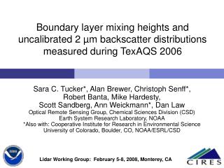
Boundary layer mixing heights and uncalibrated 2 µm backscatter distributions measured during TexAQS 2006. Sara C. Tucker*, Alan Brewer, Christoph Senff*, Robert Banta, Mike Hardesty, Scott Sandberg, Ann Weickmann*, Dan Law Optical Remote Sensing Group, Chemical Sciences Division (CSD)

E N D
Boundary layer mixing heights and uncalibrated 2 µm backscatter distributions measured during TexAQS 2006 Sara C. Tucker*, Alan Brewer, Christoph Senff*,Robert Banta, Mike Hardesty, Scott Sandberg, Ann Weickmann*, Dan Law Optical Remote Sensing Group, Chemical Sciences Division (CSD) Earth System Research Laboratory, NOAA *Also with: Cooperative Institute for Research in Environmental Science University of Colorado, Boulder, CO, NOAA/ESRL/CSD Lidar Working Group: February 5-8, 2008, Monterey, CA Working Group on Space-Based Lidar Winds, Monterrey, CA February 4-7, 2008
0 0 4 min conical scans (1, 7 and 45 degree elevations) 6 min Zenith Stare 6 min Zenith Stare 5 min Elevation Scans 15 15 45 45 HRDL scan sequence Scan sequence repeats every 15 repeats every 15 minutes minutes 30 30 HIGH RESOLUTION DOPPLER LIDAR (HRDL) HRDL Parameters RV Brown HRDL
Mixing Height estimation is finished and results now being used for: Mixing Ratios (e.g. for secondary formaldehyde production) Small scale WRF modeling validation Atmospheric scientist “buy-in” for Doppler lidar products Analysis of the effects of the relationship of the nocturnal LLJ to Houston ozone levels. Statistics on relative aerosol backscatter profiles (Size distribution data not yet available to generate actual 2 micron backscatter). HRDL analysis – what’s new?
Lidar profiles and methods for 15 minute MIXING HEIGHT ESTIMATION • hσ fromcomposite velocity variance σV2profiles (horizontal σH2 and vertical σw2) • hA from profiles of relative aerosol backscatter SRAB • hspd, hdir, and hvec from horizontal mean wind profiles
MIXING HEIGHT PRODUCT • Boundary layer: That layer of the atmosphere in turbulent connection with the surface of the earth, on time scales of about an hour (Stull, 1988) • hσ, hspd, hdir, hvec, and hA are all candidates for MH – but hσ is the most appropriate since it directly represents turbulence. • The others are related to turbulence as the cause (shear) or effect (aerosol gradient) and so may be used when hσ is not available.
Vertical velocity variance σw2 profiles are calculated using vertical velocity data from each vertical stare period. These can then be displayed using color for amplitude.
Mixing or Mixed? The top of the aerosol layer does not always correspond to the mixing height.
Data from HRDL elevation scans are binned and used to calculate estimates of horizontal variance σH2 that comprise the lowest 300 meters of the σV2 profile Horizontal velocity variance drops below threshold at the same altitude as the wind speed shear profile. Sonde profiles indicate a 200 m mixed layer
WRF model validation Gulf of Mexico Gulf of Mexico andGalveston Bay
MIXING HEIGHT ESTIMATION: Summary (For TexAQS 2006 data) • High variability over land – doesn’t match aerosol profiles, • Less variability (in mixing or aerosol layers) over Gulf • More clouds over Gulf • Velocity variance σV2profiles used here for MH later for TKE to feed into models
Sunrise Sunrise Sunset Sunset Nocturnal Low level jet Speed shear Northerly and Northwesterly flow aloft South/South-easterly flow South-Southwesterly flow Southeasterly Log scale intensity Turbulence follows a diurnal cycle due to land influence Turbulence is fairly constant, until late afternoon at which point the ship is near the shipping lanes outside of Galveston. Sea breeze
Distributions in relative aerosol backscatter (above threshold) Inland
Distributions in relative aerosol backscatter (above threshold) Gulf of Mexico
Can’t pull signal out from below noise floor. CNR mismatch Refractive turbulence effects. Changes in noise floor: clouds in noise-bins, RF noise, etc. 5000 4000 3000 2000 1000 0 -20 -15 -10 -5 0 5 10 15 20 Backscatter Inversion
Next… • Implement more thorough CNR filtering and fitting algorithms for backscatter inversion • Integrate size distribution data into Mie backscatter model. • Compare HRDL data with in-situ-based calculations of backscatter • Variance profiles TKE profiles: integrate into CNR models • Quantify the effects of these conditions on space-based lidar CNR & wind estimates.
Particle size distributions: concentrations and backscatter Likely hard target returns
2µm Backscatter: Caveats • CNR fit depends on: • Refractive turbulence • Transmission/extinction (estimated in Mie models) • Ship plume – strong refractive turbulence • Possible long-term system changes due to high vibration • Mie scattering models still “young” • Particle refractive index is highly composition dependent): Incorporate variable mass fractions of Ammonium Sulfate, Sea Salt, and Dust
Distributions in relative aerosol backscatter (above threshold) Inland
Distributions in relative aerosol backscatter (above threshold) Gulf of Mexico
Lidar profiles and methods for 15 minute MIXING HEIGHT ESTIMATION • hσ- Find the height at which surface-connected velocity variance falls below 0.04 m2s-2. • hRAB - Use the Haar wavelet method to detect gradient at top of surface-based aerosol layer. • hspd - If speed shear greater than 0.05 s-1 is present, find the altitude at which the shear falls below 0.01 s-1. • hdir - If directional shear greater than 0.05 °m-1 is present, find the altitude at which the shear falls below 0.01 °m-1 . • hvec - If vector shear greater than 2 s-1 is present, find the altitude at which the shear falls below 0.01 s-1.
Accuracy – how far off is the mean? Bias. Precision – what is the standard deviation of the measurements? Averaging more ACFs or Spectra typically means better precision – but may not mean the results are accurate. Accuracy and Precision Low accuracy, high precision High accuracy, low precision
Distributions in relative aerosol backscatter (above threshold) All locations Gulf of Mexico
Distributions in relative aerosol backscatter (above threshold) Inland/Bay Gulf of Mexico