Download

1 / 58
580 likes | 604 Views
This lecture series delves into the signals from particle jets, jet algorithms, calibration strategies, and refinement techniques at the Large Hadron Collider (LHC). Gain insights into jet response and reconstruction processes, and understand the experimentalist's perspective on jetology and detector signal measurements. Explore the challenges and strategies in jet reconstruction, as well as the importance of accurate jet calibration for studying collision dynamics. Join to deepen your knowledge of particle physics and the cutting-edge research at the LHC.

E N D
Jet Reconstruction at the LHC(Lecture 1) Peter Loch University of Arizona Tucson, Arizona, USA (loch@physics.arizona.edu)
The Large Hadron Collider (LHC) • Machine • Occupies old LEP tunnel at CERN, Geneva, Switzerland & France • About 27 km long • 50-100m underground • 1232 bending magnets • 392 focusing magnets • All superconducting • ~96 tons of He for ~1600 magnets • Beams (design) • pp collider • 7 TeV on 7 TeV (14 TeV collision energy) • Luminosity 1034 cm-2s-1 • 2808 x 2808 bunches • Bunch crossing time 25 ns (40 MHz) • ~23 pp collisions/bunch crossing • Heavy ion collider (Pb) • Collision energy 1150 TeV (2.76 TeV/nucleon)
Overview • Lecture 1 (Saturday, October 4th, 2008, 12:30-13:30): Signals from particle jets • Experimentalist’s view on jets • Jet response of a non-compensating calorimeter • Brief view at the ATLAS & CMS detectors • Calorimeter signal reconstruction: cells, towers, clusters • Lecture 2 (Sunday, October 5th, 2008, 12:30-13:30): Jet algorithms and reconstruction • Physics environment for jet reconstruction at LHC • Jet algorithms and reconstruction guidelines • Jet calibration strategies • Jet Reconstruction Performance • Lecture 3 (Sunday, October 5th, 2008, 17:00-18:00): Refinement of jet reconstruction at LHC • Refined calibration using other detectors • Tagging jets from pile-up • The origin of jets: masses and shapes • AOB
Lecture 1: Experimentalist’s view on jets “Jetology 101” • What are jets for experimentalists? • A bunch of particles generated by hadronization of a common source • Quark, gluon fragmenation • As a consequence, the particles in this bunch have correlated kinematic properties • The interacting particles in this bunch generated an observable signal in a detector • Protons, neutrons, pions, photons, electrons, muons, other particles with laboratory lifetimes >~10ps, and the corresponding anti-particles • The non-interacting particles do not generate a directly observable signal • Neutrinos, mostly • The real answer was of course given in Michael Peskin’s lecture, of course! • What is jet reconstruction, then? • Model: attempt to collect the final state particles described above into objects (jets) representing the original parton kinematic • Re-establishing the correlations • Experiment: attempt to collect the detector signals from these particles to measure their original kinematics • Usually not the parton!
Lecture 1: Experimentalist’s view on jets Experiment (“Nature”)
Particles MB MB MB Lecture 1: Experimentalist’s view on jets Experiment (“Nature”) Modeling Particle Jets Generated Particles Particle Jets Jet Finding Stable Particles Decays Fragmentation UE Multiple Interactions
Stable Particles Lecture 1: Experimentalist’s view on jets Experiment (“Nature”) Modeling Calorimeter Jets Reconstructed Jets Identified Particles Jet Finding Reconstructed Calorimeter Signals Signal Reconstruction Raw Calorimeter Signals Detector Simulation
Lecture 1: Experimentalist’s view on jets Experiment (“Nature”) Measuring Calorimeter Jets Reconstructed Jets Identified Particles Jet Finding Reconstructed Calorimeter Signals Signal Reconstruction Raw Calorimeter Signals Measurement Observable Particles
Lecture 1: Experimentalist’s view on jets Experiment (“Nature”) Jet Reconstruction Challenges longitudinal energy leakage detector signal inefficiencies (dead channels, HV…) pile-up noise from (off- and in-time) bunch crossings electronic noise calo signal definition (clustering, noise suppression…) dead material losses (front, cracks, transitions…) detector response characteristics (e/h ≠ 1) jet reconstruction algorithm efficiency lost soft tracks due to magnetic field added tracks from underlying event added tracks from in-time (same trigger) pile-up event jet reconstruction algorithm efficiency physics reaction of interest (interaction or parton level)
Lecture 1: Experimentalist’s view on jets Jet Reconstruction • Experimental goal • Find the best “picture” of the final state representing the collision dynamics behind a given event • Best reconstruction of fragmented hard scattered parton and general event energy flow • “Resolution” requirements for this picture depend on physics question asked • Reconstruct source of jet • Sequential process • Input signal selection • Get the best signals out of your detector on a given scale • Preparation for jet finding • Suppression/cancellation of “unphysical” signal objects with E<0 (due to noise) • Possibly event ambiguity resolution (remove reconstructed electrons, photons, taus,… from detector signal) • Pre-clustering to speed up reconstruction (not needed as much anymore) • Jet finding • Apply your jet finder of choice • Jet calibration • Depending on detector, jet finder choices, references… • Jet selection • Apply cuts on kinematics etc. to select jets of interest or significance • Objective • Reconstruct particle level features • Test models and extract physics
Lecture 1: Experimentalist’s view on jets Jet Signal Detection • Calorimeters are the detectors of choice • Generate signals from charged and neutral particles in jets • Tracking devices only sensitive to charged particles • Full absorption detectors • All energy of the original particle deposited within calorimeter • Generate signals proportional to energy deposit • Segmented readout • Collection energy in (small) volumes allows reconstruction of the particle direction • Spatial energy distribution hints at incoming particle nature • Overall detector contributes to detection efficiency • Magnetic field • Often solenoid field in inner detector cavity in front of calorimeters • Leads to jet energy losses due to bending of charged particles away from the calorimeter (low pT, no calorimeter signal at all) or away from the jet • Inactive materials • Energy losses in inner detector and its services and support (from point of calorimetry) • Energy losses in mechanical structures insides (support beams, internal transition regions etc.) and outside the calorimeter (cryostat walls etc.)
Lecture 1: Jet response of non-compensating calorimeters Calorimeter Basics (1) • Full absorption detector • Idea is to convert incoming particle energy into detectable signals • Light or electric current • Should work for charged and neutral particles • Exploits the fact that particles entering matter deposit their energy in particle cascades • Electrons/photons in electromagnetic showers • Charged pions, protons, neutrons in hadronic showers • Muons do not shower at all in general • Principal design challenges • Need dense matter to absorb particles within a small detector volume • Lead for electrons and photons, copper or iron for hadrons • Need “light” material to collect signals with least losses • Scintillator plastic, nobel gases and liquids • Solution I: combination of both features • Crystal calorimetry, BGO • Solution II: sampling calorimetry
Lecture 1: Jet response of non-compensating calorimeters Calorimeter Basics (2) • Sampling calorimeters • Use dense material for absorption power… • No direct signal • …in combination with highly efficient active material • Generates signal • Consequence: only a certain fraction of the incoming energy is directly converted into a signal • Typically 1-10% • Signal is therefore subjected to sampling statistics • The same energy loss by a given particle type may generate different signals • Limit of precision in measurements • Need to understand particle response • Electromagnetic and hadronic showers
Lecture 1: Jet response of non-compensating calorimeters Electromagnetic Calorimeter Signals • Electromagnetic showers • Particle cascade generated by electrons/positrons and photons in matter • Developed by brems-strahlung & pair-production • Compact signal • Regular shower shapes • Small shower-to-shower fluctuations • Strong correlation between longitudinal and lateral shower spread • Well measured in sampling calorimeters • Signal directly proportional to deposited energy • Signal resolution nearly completely due to sampling fluctuations
Grupen, Particle Detectors Cambridge University Press (1996) Lecture 1: Jet response of non-compensating calorimeters Hadronic Showers • Hadronic cascades • Particle cascade generated in matter by hadron-nucleon collisions in nucleus • Driving force for shower development is strong interaction • ~200 possible processes with <1% probability each! • Intrinsic electromagnetic showers from π0 production in inelastic hadronic interaction Hadron-nucleus interaction: • Fast component from internal hadron-nucleon cascades produce more hadrons continues shower development • Energy in slow nuclear phase with nuclear fission or break-up, and evaporation (de-exitation) lost for shower developement
Lecture 1: Jet response of non-compensating calorimeters Hadronic Shower Characteristics • Hadronic signals • Signal only from ionization by charged particles and intrinsic electromagnetic showers • Large energy losses without signal generation • Binding energy losses • Escaping energy/slow particles (neutrinos/neutrons) • Signal depends on size of electromagnetic component • Energy invested in neutral pions lost for further hadronic shower developement • Fluctuating significantly shower-by-shower • Weakly depending on incoming hadron energy • Consequence: non-compensation • Hadrons generate less signal than electrons depositing the same energy
Electromagnetic Compact Growths in depth ~log(E) Longitudinal extension scale is radiation length X0 Distance in matter in which ~50% of electron energy is radiated off Photons 9/7 X0 Strong correlation between lateral and longitudinal shower development Small shower-to-shower fluctuations Very regular development Can be simulated with high precision 1% or better, depending on features Hadronic Scattered, significantly bigger Growths in depth ~log(E) Longitudinal extension scale is interaction length λ Average distance between two inelastic interactions in matter Varies significantly for pions, protons, neutrons Weak correlation between longitudinal and lateral shower development Large shower-to-shower fluctuations Very irregular development Can be simulated with reasonable precision ~2-5% depending on feature Lecture 1: Jet response of non-compensating calorimeters Shower Parameters
Lecture 1: Jet response of non-compensating calorimeters Hadronic Signal Composition (1) Single hadron response: with intrinsic electromagnetic energy fraction in hadronic showers parametrized as*: *D.Groom et al., NIM A338, 336-347 (1994)
Lecture 1: Jet response of non-compensating calorimeters Hadron Signal Composition (2) Observable provides experimental access to characteristic calorimeter variables in pion testbeams, like e/h, by fitting the energy dependence of the pion signal in testbeams: e/h is often constant, example: in both H1 and ATLAS about 50% of the energy in the hadronic branch generates a signal independent of the energy itself
Lecture 1: Jet response of non-compensating calorimeters Jet Signal Composition Jet response with perfect acceptance (all particles detected): Jet energy fractions from fragmentation functions: Fragmentation well measured at LEP – extrapolation to much higher energy jets not obvious jet energy hardest parton pT>280 GeV jet transverse energy jet rapidity
Lecture 1: Jet response of non-compensating calorimeters Ideal Jet Response • Assume all particles in jet contribute to signal • Not really true, see later • Expect primary photon content to increase jet signal compared to pion signal • Expectation too naïve • low energetic particles may not reach calorimeter at all • Realistic response evaluation needs acceptance folded in! Response Ratio Energy (GeV)
Lecture 1: Jet response of non-compensating calorimeters Calorimeter Acceptance Not all incoming energy deposited in calorimeter due to upstream material losses (depend on the particle type and material) Basic energy scale signal depends on particle type, deposited energy and signal characteristics of calorimeter (noise etc.); Detection thresholds on incoming particle energy – no precision measurement possible below this!
Jets are bundles of particles ~25% initial photons Hadronic particles include mostly pions, kaons, protons and their anti-particles Different response! Jet response in non-compensating calorimeters Jet signal depends on fragmentation/particle content Significant jet-to-jet response variations due to more or less photons Lecture 1: Jet response of non-compensating calorimeters Jet Response To Jet Energy Reconstruction only source of signal!
Lecture 1: Jet response of non-compensating calorimeters Limitations Of Simple Models • Jet response is complex • Need to understand electron/photon and hadron response of calorimeter • Also need to understand acceptance for each particle type • Signal thresholds • Overlapping showers in jets may enhance acceptance for low energetic particles if compared to isolated particles • Jet particle content/fragmentation not easily accessible in hadron colliders • Cannot analytically fold single particle response with fragmentation to understand experimental signals • Large fluctuations in particle composition • Large shower signal fluctuations for hadrons • Net effect on jets depends on fragmentation! • Need physics and detector simulation to understand jet response!!
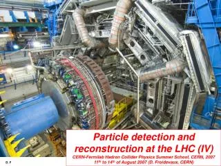
Lecture 1: ATLAS & CMS Detectors ATLAS: A General Purpose Detector For LHC Total weight : 7000 t Overall length: 46 m Overall diameter: 23 m Magnetic field: 2T solenoid + toroid
Lecture 1: ATLAS & CMS Detectors CMS: A General Purpose Detector For LHC Total weight: 12500 t Overall length: 22 m Overall diameter: 15 m Magnetic field: 4T solenoid
Lecture 1: ATLAS & CMS Detectors Typical Detector Features • Hermetic coverage over a wide angular range • Efficient missing transverse energy reconstruction due to large coverage in pseudo-rapidity • Very forward detection of particles and jets produced in pp collisions • High particle reconstruction efficiency • Important for final state reconstruction and classification • Relative energy resolution for electrons, photons and muons is 2-4%
EM Barrel EMB EM Endcap EMEC Hadronic Endcap Tile Barrel Forward Tile Extended Barrel Lecture 1: ATLAS & CMS Detectors The ATLAS Calorimeters Electromagnetic Barrel || < 1.4 Electromagnetic EndCap 1.375 < || < 3.2 Hadronic Tile || < 1.7 Hadronic EndCap 1.5 < || < 3.2 Forward Calorimeter 3.2 < || < 4.9 Varied granularity Varied technologies Overlap/crack regions ~200,000 readout cells
Lecture 1: ATLAS & CMS Detectors Electromagnetic Calorimetry • Highly segmented lead/liquid argon accordion • No azimuthal cracks • 3 depth segments • + pre-sampler (limited coverage) • Strip cells in 1st layer • Very high granularity in pseudo-rapidity • Deep cells in 2nd layer • High granularity in both directions • Shallow cells in 3rd layer Electromagnetic Barrel
Lecture 1: ATLAS & CMS Detectors Hadronic Calorimetry • Tile calorimeter • Iron/scintillator tiled readout • 3 depth segments • Quasi-projective readout cells • First two layers: • Third layer • Very fast light collection • ~50 ns • Dual fiber readout for each channel
Electromagnetic “Spanish Fan” accordion Highly segmented with up to three longitudinal segments Hadronic liquid argon/copper calorimeter Parallel plate design Four longitudinal segments Quasi-projective cells Lecture 1: ATLAS & CMS Detectors EndCap Calorimeters
FCal3 FCal1 FCal2 Lecture 1: ATLAS & CMS Detectors Forward Calorimeters • Design features • Compact absorbers • Small showers • Tubular thin gap electrodes • Suppress positive charge build-up (Ar+) in high ionization rate environment • Stable calibration • Rectangular non-projective readout cells • Electromagnetic FCal1 • Liquid argon/copper • Gap ~260 μm • Hadronic FCal2 • Liquid argon/tungsten • Gap ~375 μm • Hadronic FCal3 • Liquid argon/tungsten • Gap ~500 μm
Lecture 1: ATLAS & CMS Detectors ATLAS Calorimeter Summary • Non-compensating calorimeters • Electrons generate larger signal than pions depositing the same energy • Typically e/π ≈ 1.3 • High particle stopping power over whole detector acceptance |η|<4.9 • ~26-35 X0electromagnetic calorimetry • ~ 10 λ total for hadrons • Hermetic coverage • No significant cracks in azimuth • Non-pointing transition between barrel, endcap and forward • Small performance penalty for hadrons/jets
Lecture 1: Calorimeter Signal Reconstruction Signal Collection
Lecture 1: Calorimeter Signal Reconstruction Signal Formation in ATLAS (Example) • Slow signal formation • ~450 ns drift time @ 1 kV/mm electric field • High bunch crossing (collision) frequency at LHC • 40 MHz/every 25 ns • Shape signal electronically • Make time integrated average of all signals 0 • Suppresses signal history, no signal pile-up • Bi-polar shaping with fast rising edge • Peak of shaped pulse is measure of initial current reading out (digitize) 5 samples sufficient!
Lecture 1: Calorimeter Signal Reconstruction Online Signal Channel Processing Correction & calibration sequence is example only! Order and applicable factors depend on calorimeter sub-system (electrode structure, readout organization…)
Lecture 1: Calorimeter Signal Reconstruction Calorimeter Cells • Smallest signal collection volume • Defines resolution of spatial structures • Each is read out independently • Individual cell signals • Sensitive to noise • Fluctuations in electronics gain and shaping • Time jitters • Physics sources like multiple interactions • Hard to calibrate • No measure to determine if electromagnetic or hadronic, i.e. no handle to estimate e/h from single cell alone • Need signal neighbourhood to calibrate • Basic energy scale • Use electron calibration to establish basic energy scale for cell signals • Cell geometry • Often pointing to the nominal collision vertex • Lateral sizes scale with pseudo-rapidity and azimuthal angular opening
Imposes regular grid view on event ( ) Motivated by event ET flow Natural for trigger! Calorimeter cell signals are summed up in tower bins Default: no cell selection, all cells are included Indiscriminatory signal sum includes cells without any true signal at all Sum typically includes geometrical weight Towers have fixed direction Massless four-momentum representation on electro- magnetic energy scale Lecture 1: Calorimeter Signal Reconstruction Collecting Cells: Towers projective cells non-projective cells
Lecture 1: Calorimeter Signal Reconstruction Topological Cell Clusters • Motivation • Attempt reconstruction of individual particle showers • Reconstruct 3-dim clusters of cells with correlated signals • Use shape of these clusters to locally calibrate them • Explore differences between electromagnetic and hadronic shower development and select best suited calibration • Supress noise with least bias on physics signals • Often less than 50% of all cells in an event with “real” signal • Implementation • Find seed with significant signal above primary seed threshold S • Signal significance is signal-over-noise (absolute) • Collect all neighbouring cells (in 3-d) with signals with significance above basic threshold P • If neighbouring cells have signal above secondary seed N, collect neighbours of neighbours if they have significance above P • Analyze clusters for local signal maxima and split if more than one found • In 3-d, again • Note that very low signal cells can survive “effective” cell signal significance selection with this algorithm if larger signal in vicinity
cluster candidate #1 #3? cluster candidate #2 Lecture 1: Calorimeter Signal Reconstruction Topological Cell Clusterscont’d
Lecture 1: Calorimeter Signal Reconstruction Calorimeter Jet Signals: It’s All In The Pictures…
RD3 note 41, 28 Jan 1993 Lecture 1: Calorimeter Signal Reconstruction Hadronic Cluster Calibration • Local approach (cluster context) • Calibrate calorimeter signal first • Provides calibration for all signals without need for jet context • Separate electromagnetic from hadronic signals • Topological clustering/energy blob recon- struction • Cluster shape analysis explores differences between electromagnetic and hadronic shower development • Compactness of electromagnetic shower • Attempt to only calibrate hadronic clusters • Non-compensation only issue for hadronic showers • Absorb particle or jet signal variations due to algorithms, size, physics environment into corrections • Factorization possible • Jet context corrections not applied to other hadronic objects • Cannot completely factorize calibration and corrections • Correlation between inactive material energy losses and effective e/h in calorimeters, for example
Lecture 1: Calorimeter Signal Reconstruction Local Hadronic Calibration CaloCluster (em scale) Cluster Classification electromagnetic hadronic Hadronic Calibration Dead Material Corrections Dead Material Corrections Out-of-cluster Corrections Out-of-cluster Corrections CaloCluster (calibrated)
Lecture 1: Calorimeter Signal Reconstruction Cell Signal Weighting In ATLAS • Weights are extracted from simulations • Signals and deposited energies from single charged pion MC • Weights are calculated as function of cluster & cell variables • Signal environment used as additional indicator of hadronic character
Lecture 1: Calorimeter Signal Reconstruction Local Hadronic Calibration Summary • Attempt to calibrate hadronic calorimeter signals in smallest possible signal context • Topological clustering implements noise suppression with least bias signal feature extraction • No bias towards a certain physics analysis • Good common signal base for all hadronic final state objects • Jets, missing Et, taus • Factorization of cluster calibration • Cluster classification largely avoids application of hadronic calibration to electromagnetic signal objects • Low energy regime challenging • Signal weights for hadronic calibration are functions of cluster and cell parameters and variables • Cluster energy and direction • Cell signal density and location (sampling layer) • Dead material and out of cluster corrections are independently applied
Lecture 1: Calorimeter Signal Reconstruction From This Lecture: • Calorimeters are signal processors for incoming particles • They generate an image of particles they are sensitive to in the collision event • The image is distorted due to environment (physics and detector) • Calorimeter signal reconstruction is the attempt to improve the resolution of this image • Attempt to unfold the distortions by signal definition, possibly including identification of significant objects • Best choice for unfolding strategy may depend on physics question • Two signal definitions (e.g., towers and clusters) allow evaluation of systematic uncertainties • We will explore this further in the 2nd lecture on Sunday!