Download
1 / 37
370 likes | 389 Views
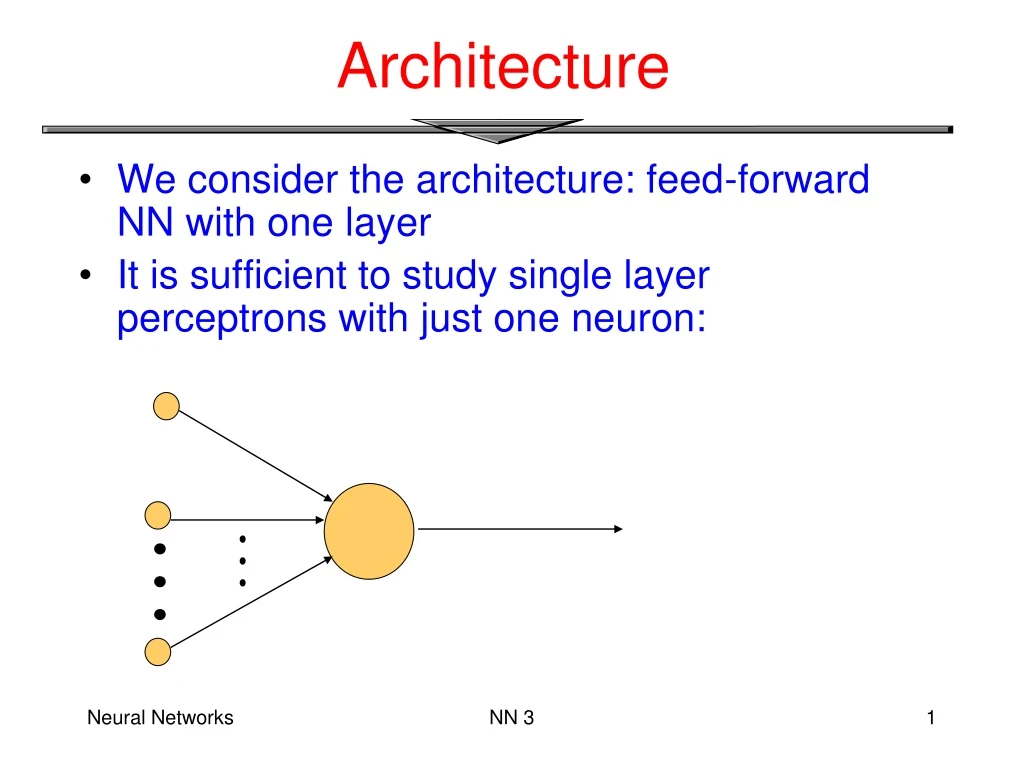
Architecture. We consider the architecture: feed-forward NN with one layer It is sufficient to study single layer perceptrons with just one neuron:. Single layer perceptrons. Generalization to single layer perceptrons with more neurons is easy because:.

E N D
Architecture • We consider the architecture: feed-forward NN with one layer • It is sufficient to study single layer perceptrons with just one neuron: NN 3
Single layer perceptrons • Generalization to single layer perceptrons with more neurons is easy because: • The output units are independent among each other • Each weight only affects one of the outputs NN 3
b (bias) x1 w1 v y x2 w2 (v) wn xn Perceptron: Neuron Model • The (McCulloch-Pitts) perceptron is a single layer NN with a non-linear , the sign function NN 3
Perceptron for Classification • The perceptron is used for binary classification. • Given training examples of classes C1, C2 train the perceptron in such a way that it classifies correctly the training examples: • If the output of the perceptron is +1 then the input is assigned to class C1 • If the output is -1 then the input is assigned to C2 NN 3
Perceptron Training • How can we train a perceptron for a classification task? • We try to find suitable values for the weights in such a way that the training examples are correctly classified. • Geometrically, we try to find a hyper-plane that separates the examples of the two classes. NN 3
Perceptron Geometric View The equation below describes a (hyper-)plane in the input space consisting of real valued m-dimensional vectors. The plane splits the input space into two regions, each of them describing one class. decision region for C1 x2 w1x1 + w2x2 + w0 >= 0 decision boundary C1 x1 C2 w1x1 + w2x2 + w0< 0 NN 3
Example NN 3
Example • How to train a perceptron to recognize this 3? • Assign –1 to weights of input values that are equal to -1, +1 to weights of input values that are equal to +1, and –63 to the bias. • Then the output of the perceptron will be 1 when presented with a “prefect” 3, and at most –1 for all other patterns. NN 3
Example NN 3
Example • What if a slightly different 3 is to be recognized, like the one in the previous slide? • The original 3 with one bit corrupted would produce a sum equal to –1. • If the bias is set to –61 then also this corrupted 3 will be recognized, as well as all patterns with one corrupted bit. • The system has been able to generalize by considering only one example of corrupted pattern! NN 3
Perceptron: Learning Algorithm • Variables and parameters at iteration n of the learning algorithm: x(n) = input vector = [+1, x1(n), x2(n), …, xm(n)]T w(n) = weight vector = [b(n), w1(n), w2(n), …, wm(n)]T b(n) = bias y(n) = actual response d(n) = desired response = learning rate parameter NN 3
The fixed-increment learning algorithm n=1; initializew(n) randomly; while (there are misclassified training examples) Select a misclassified augmented example (x(n),d(n)) w(n+1) = w(n) + d(n)x(n); n = n+1; end-while; = learning rate parameter (real number) NN 3
Consider the 2-dimensional training set C1 C2, C1 = {(1,1), (1, -1), (0, -1)} with class label 1 C2 = {(-1,-1), (-1,1), (0,1)} with class label -1 Train a perceptron on C1 C2 Example NN 3
A possible implementation Consider the augmented training set C’1 C’2, with first entry fixed to 1 (to deal with the bias as extra weight): (1, 1, 1), (1, 1, -1), (1, 0, -1) ,(1,-1, -1), (1,-1, 1), (1,0,1) Replace x with -x for all x C2’ and use the following update rule: Epoch = application of the update rule to each example of the training set. Execution of the learning algorithm terminates when the weights do not change after one epoch. NN 3
Execution • the execution of the perceptron learning algorithm for each epoch is illustrated below, with w(1)=(1,0,0), =1, and transformed inputs (1, 1, 1), (1, 1, -1), (1,0, -1), (-1,1, 1), (-1,1, -1), (-1,0, -1) End epoch 1 NN 3
Execution End epoch 2 At epoch 3 no weight changes. (check!) stop execution of algorithm. Final weight vector: (0, 2, -1). decision hyperplane is 2x1 - x2 = 0. NN 3
Result x2 1 - - + Decision boundary: 2x1 - x2 = 0 C2 x1 -1 1 2 1/2 w -1 C1 - + + NN 3
Suppose the classes C1, C2are linearly separable (that is, there exists a hyper-plane that separates them). Then the perceptron algorithm applied to C1 C2 terminates successfully after a finite number of iterations. Proof: Consider the set C containing the inputs of C1 C2transformed by replacing x with -x for each x with class label -1. For simplicity assume w(1) = 0, = 1. Let x(1) … x(k) Cbe the sequence of inputs that have been used after k iterations. Then w(2) = w(1) + x(1) w(3) = w(2) + x(2) w(k+1) = x(1) + … + x(k) w(k+1) = w(k) + x(k) Termination of the learning algorithm NN 3
Perceptron Limitations • A single layer perceptron can only learn linearly separable problems. • Boolean AND function is linearly separable, whereas Boolean XOR function (and the parity problem in general) is not. 20
Linear Separability Boolean AND Boolean XOR 21
Perceptron Limitations Linear Decision Boundary Linearly Inseparable Problems 22
Perceptron Limitations • XOR problem: What if we use more layers of neurons in a perceptron? • Each neuron implementing one decision boundary and the next layer combining the two? What could be the learning rule for each neuron? => Multilayer networks and the backpropagation learning 23
Perceptrons ( in the most specific case, they refer to single layer perceptrons)can learn many Booleanfunctions: AND, OR, NAND, NOR, but not XOR x1 AND: W1=0.5 Σ W2=0.5 W0 = -0.8 x2 X0=1 24
More than one layer of perceptrons (with a hardlimiting activation function) can learn any Boolean function • However, a learning algorithm for multi-layer perceptrons has not been developed until much later - backpropagation algorithm (replacing the hardlimiter with a sigmoid activation function) 25
Adaline-I • Adaline (adaptive linear element) is an adaptive signal processing/pattern classification machine that uses LMS algorithm. Developed by Widrow and Hoff • Inputs x are either -1 or +1, threshold is between 0 and 1 and output is either -1 or +1 • LMS algorithm is used to determine the weights. Instead of using the output y, the net input u is used in the error computation, i.e., e = d – u (because y is quantized in the Adaline) NN 3
Adaline: Adaptive Linear Element -II • When the two classes are not linearly separable, it may be desirable to obtain a linear separator that minimizes the mean squared error. • Adaline (Adaptive Linear Element): • uses a linear neuron model and • the Least-Mean-Square (LMS) learning algorithm • useful for robust linear classification and regression For an example (x,d) the error e(w) of the network is and the squared error is NN 3
Adaline (1) 28 NN 3
Adaline-III • The total error E_tot is the mean of the squared errors of all the examples. • E_tot is a quadratic function of the weights, whose derivative exists everywhere. • Incremental gradient descent may be used to minimize E_tot.. • At each iteration LMS algorithm selects an example and decreases the network error E of that example, even when the example is correctly classified by the network. NN 3
Wiener-Hopf Equations • The goal is to find the optimum weights that minimizes the difference between the system output y and some desired response d in the mean-square sense • System equations y = Σk=1 wkxk e = d – y • Performance measure or cost function J = 0.5E[e2] ; E = expectation operator • Find the optimum weights for which J is a minimum NN 3
LMS Algorithm (2) NN 3
Gradient direction Gradient Descent Example • Gradient is the slope of the line, formally F’(x(t)) • Gradient Descent Algorithm: x(t+1) = x(t) – F’(x(t)) • At current position, the slope (F’(x(t)) is positive (going upwards) • The searcher therefore goes downhill from here since we subtract F’(x(t)) from our current position (move leftwards) • If the step size (constant ) is too large the search might overshoot and oscillate around the optimum for a while • Eventually the searcher stops at a minima where the gradient is zero x(t) NN 3
Incremental Gradient Descent • start from an arbitrary point in the weight space • the direction in which the error E of an example (as a function of the weights) is decreasing most rapidly is the opposite of the gradient of E: • take a small step (of size ) in that direction NN 3
Weights Update Rule • Computation of Gradient(E): • Delta rule for weight update: NN 3
LMS learning algorithm n=1; initializew(n) randomly; while (E_tot unsatisfactory and n<max_iterations) Select an example (x(n),d(n)) n = n+1; end-while; = learning rate parameter (real number) A modification uses NN 3