Download
1 / 294
2.94k likes | 3.05k Views
These notes are intended for use by students in CS1501 at the University of Pittsburgh and no one else These notes are provided free of charge and may not be sold in any shape or form

E N D
These notes are intended for use by students in CS1501 at the University of Pittsburgh and no one else • These notes are provided free of charge and may not be sold in any shape or form • These notes are NOT a substitute for material covered during course lectures. If you miss a lecture, you should definitely obtain both these notes and notes written by a student who attended the lecture. • Material from these notes is obtained from various sources, including, but not limited to, the following: • Algorithms in C++ by Robert Sedgewick • Introduction to Algorithms, by Cormen, Leiserson and Rivest • Various Java and C++ textbooks
Goals of Course • Definitions: • Offline Problem: • We provide the computer with some input and after some time receive some acceptable output • Algorithm • A step-by-step procedure for solving a problem or accomplishing some end • Program • an algorithm expressed in a language the computer can understand • An algorithm solves a problem if it produces an acceptable output on EVERY input
Goals of Course • Goals of this course: • To learn how to convert (nontrivial) algorithms into programs • Often what seems like a fairly simple algorithm is not so simple when converted into a program • Other algorithms are complex to begin with, and the conversion must be carefully considered • Many issues must be dealt with during the implementation process • Let's hear some
Goals of Course • To see and understand differences in algorithms and how they affect the run-times of the associated programs • Many problems can be solved in more than one way • Different solutions can be compared using many factors • One important factor is program run-time • Sometimes a better run-time makes one algorithm more desirable than another • Sometimes a better run-time makes a problem solution feasible where it was not feasible before • However, there are other factors for comparing algorithms • Let's hear some
Algorithm Analysis • Determine resource usage as a function of input size • Which resources? • Ignore multiplicative constants and lower order terms • Why? • Measure performance as input size increases without bound (toward infinity) • Asymptotic performance • Use some standard measure for comparison • Do we know any measures?
Algorithm Analysis • Big O • Upper bound on the asymptotic performance • Big Omega • Lower bound on the asymptotic performance • Theta • Upper and lower bound on the asymptotic performance – Exact bound • Compare on the board • So why would we ever use Big O? • Theta is harder to show in some cases • Lower bounds are typically harder to show than upper bounds • So sometimes we can just determine the upper bound
Algorithm Analysis • So is algorithm analysis really important? • Yes! Different algorithms can have considerably different run-times • Sometimes the differences are subtle but sometimes they are extreme • Let's look at a table of growth rates on the board • Note how drastic some of the differences are for large problem sizes
Algorithm Analysis • Consider 2 choices for a programmer • Implement an algorithm, then run it to find out how long it takes • Determine the asymptotic run-time of the algorithm, then, based on the result, decide whether or not it is worthwhile to implement the algorithm • Which choice would you prefer? • Discuss • The previous few slides should be (mostly) review of CS 0445 material
Exhaustive Search • Idea: • We find a solution to a problem by considering (possibly) all potential solutions and selecting the correct one • Run-time: • The run-time is bounded by the number of possible solutions to the problem • If the number of potential solutions is exponential, then the run-time will be exponential
Exhaustive Search • Example: Hamiltonian Cycle • A Hamiltonian Cycle (HC) in a graph is a cycle that visits each node in the graph exactly one time • See example on board and on next slide • Note that an HC is a permutation of the nodes in the graph (with a final edge back to the starting vertex) • Thus a fairly simple exhaustive search algorithm could be created to try all permutations of the vertices, checking each with the actual edges in the graph • See text Chapter 44 for more details
Exhaustive Search F A G E D B C Hamiltonian Cycle Problem A solution is: ACBEDGFA
Exhaustive Search • Unfortunately, for N vertices, there are permutations, so the run-time here is poor • Pruning and Branch and Bound • How can we improve our exhaustive search algorithms? • Think of the execution of our algorithm as a tree • Each path from the root to a leaf is an attempt at a solution • The exhaustive search algorithm may try every path • We'd like to eliminate some (many) of these execution paths if possible • If we can prune an entire subtree of solutions, we can greatly improve our algorithm runtime N!
Pruning and Branch and Bound • For example on board: • Since edge (C, D) does not exist we know that no paths with (C, D) in them should be tried • If we start from A, this prunes a large subtree from the tree and improves our runtime • Same for edge (A, E) and others too • Important note: • Pruning / Branch and Bound does NOT improve the algorithm asymptotically • The worst case is still exponential in its run-time • However, it makes the algorithm practically solvable for much larger values of N
Recursion and Backtracking • Exhaustive Search algorithms can often be effectively implemented using recursion • Think again of the execution tree • Each recursive call progresses one node down the tree • When a call terminates, control goes back to the previous call, which resumes execution • BACKTRACKING
Recursion and Backtracking • Idea of backtracking: • Proceed forward to a solution until it becomes apparent that no solution can be achieved along the current path • At that point UNDO the solution (backtrack) to a point where we can again proceed forward • Example: 8 Queens Problem • How can I place 8 queens on a chessboard such that no queen can take any other in the next move? • Recall that queens can move horizontally, vertically or diagonally for multiple spaces • See on board
8 Queens Problem • 8 Queens Exhaustive Search Solution: • Try placing the queens on the board in every combination of 8 spots until we have found a solution • This solution will have an incredibly bad run-time • 64 C 8 = (64!)/[(8!)(64-8)!] = (64*63*62*61*60*59*58*57)/40320 = 4,426,165,368 combinations (multiply by 8 for total queen placements) • However, we can improve this solution by realizing that many possibilities should not even be tried, since no solution is possible • Ex: Any solution has exactly one queen in each column
8 Queens Problem • This would eliminate many combinations, but would still allow 88 = 16,777,216 possible solutions (x 8 = 134,217,728 total queen placements) • If we further note that all queens must be in different rows, we reduce the possibilities more • Now the queen in the first column can be in any of the 8 rows, but the queen in the second column can only be in 7 rows, etc. • This reduces the possible solutions to 8! = 40320 (x 8 = 322,560 individual queen placements) • We can implement this in a recursive way • However, note that we can prune a lot of possibilities from even this solution execution tree by realizing early that some placements cannot lead to a solution • Same idea as for Hamiltonian cycle – we are pruning the execution tree
8 Queens Problem • Ex: No queens on the same diagonal • See example on board • Using this approach we come up with the solution as shown in 8-Queens handout • JRQueens.java • Idea of solution: • Each recursive call attempts to place a queen in a specific column • A loop is used, since there are 8 squares in the column • For a given call, the state of the board from previous placements is known (i.e. where are the other queens?) • If a placement within the column does not lead to a solution, the queen is removed and moved "down" the column
8 Queens Problem • When all rows in a column have been tried, the call terminates and backtracks to the previous call (in the previous column) • If a queen cannot be placed into column i, do not even try to place one onto column i+1 – rather, backtrack to column i-1 and move the queen that had been placed there • Using this approach we can reduce the number of potential solutions even more • See handout results for details
Finding Words in a Boggle Board • Another example: finding words in a Boggle Board • Idea is to form words from letters on mixed up printed cubes • The cubes are arranged in a two dimensional array, as shown below • Words are formed by starting at any location in the cube and proceeding to adjacent cubes horizontally, vertically or diagonally • Any cube may appear at most one time in a word • For example, FRIENDLY and FROSTED are legal words in the board to the right
Finding Words in a Boggle Board • This problem is very different from 8 Queens • However, many of the ideas are similar • Each recursive call adds a letter to the word • Before a call terminates, the letter is removed • But now the calls are in (up to) eight different directions: • For letter [i][j] we can recurse to • letter [i+1][j] letter [i-1][j] • letter [i][j+1] letter[i][j-1] • letter [i+1][j+1] letter[i+1][j-1] • letter [i-1][j+1] letter[i-1][j-1] • If we consider all possible calls, the runtime for this is enormous! • Has an approx. upper bound of 16! 2.1 x 10¹³
Finding Words in a Boggle Board • Naturally, not all recursive calls may be possible • We cannot go back to the previous letter since it cannot be reused • Note if we could words could have infinite length • We cannot go past the edge of the board • We cannot go to any letter that does not yield a valid prefix to a word • Practically speaking, this will give us the greatest savings • For example, in the board shown (based on our dictionary), no words begin with FY, so we would not bother proceeding further from that prefix • Execution tree is pruned here as well • Show example on board
Implementation Note • Since a focus of this course is implementing algorithms, it is good to look at some implementation issues • Consider building / unbuilding strings that are considered in the Boggle game • Forward move adds a new character to the end of a string • Backtrack removes the most recent character from the end of the string • In effect our string is being used as a Stack – pushing for a new letter and popping to remove a letter
Implementation Note • We know that Stack operations push and pop can both be done in Θ(1) time • Unless we need to resize, which would make a push linear for that operation (still amortized Θ(1) – why?) • Unfortunately, the String data type in Java stores a constant string – it cannot be mutated • So how do we “push” a character onto the end? • In fact we must create a new String which is the previous string with one additional character • This has the overhead of allocating and initializing a new object for each “push”, with a similar overhead for a “pop” • Thus, push and pop have become Θ(N) operations, where N is the length of the string • Very inefficient!
Implementation Note • For example: S = new String(“ReallyBogusLongStrin”); S = S + “g”; • Consider now a program which does many thousands of these operations – you can see why it is not a preferred way to do it • To make the “push” and “pop” more efficient (Θ(1)) we could instead use a StringBuffer (or StringBuilder) • append() method adds to the end without creating a new object • Reallocates memory only when needed • However, if we size the object correctly, reallocation need never be done • Ex: For Boggle (4x4 square) S = new StringBuffer(16);
Review of Searching Methods • Consider the task of searching for an item within a collection • Given some collection C and some key value K, find/retrieve the object whose key matches K Q K K P … Z J
Review of Searching Methods • How do we know how to search so far? • Well let's first think of the collections that we know how to search • Array/Vector • Unsorted • How to search? Run-time? • Sorted • How to search? Run-time? • Linked List • Unsorted • How to search? Run-time? • Sorted • How to search? Run-time?
Review of Searching Methods • Binary Search Tree • Slightly more complicated data structure • Run-time? • Are average and worst case the same? • So far binary search of a sorted array and a BST search are the best we have • Both are pretty good, giving O(log2N) search time • Can we possibly do any better? • Perhaps if we use a very different approach
Digital Search Trees • Consider BST search for key K • For each node T in the tree we have 4 possible results • T is empty (or a sentinel node) indicating item not found • K matches T.key and item is found • K < T.key and we go to left child • K > T.key and we go to right child • Consider now the same basic technique, but proceeding left or right based on the current bit within the key
Digital Search Trees • Call this tree a Digital Search Tree (DST) • DST search for key K • For each node T in the tree we have 4 possible results • T is empty (or a sentinel node) indicating item not found • K matches T.key and item is found • Current bit of K is a 0 and we go to left child • Current bit of K is a 1 and we go to right child • Look at example on board
Digital Search Trees • Run-times? • Given N random keys, the height of a DST should average O(log2N) • Think of it this way – if the keys are random, at each branch it should be equally likely that a key will have a 0 bit or a 1 bit • Thus the tree should be well balanced • In the worst case, we are bound by the number of bits in the key (say it is b) • So in a sense we can say that this tree has a constant run-time, if the number of bits in the key is a constant • This is an improvement over the BST
Digital Search Trees • But DSTs have drawbacks • Bitwise operations are not always easy • Some languages do not provide for them at all, and for others it is costly • Handling duplicates is problematic • Where would we put a duplicate object? • Follow bits to new position? • Will work but Find will always find first one • Actually this problem exists with BST as well • Could have nodes store a collection of objects rather than a single object
Digital Search Trees • Similar problem with keys of different lengths • What if a key is a prefix of another key that is already present? • Data is not sorted • If we want sorted data, we would need to extract all of the data from the tree and sort it • May do b comparisons (of entire key) to find a key • If a key is long and comparisons are costly, this can be inefficient
Radix Search Tries • Let's address the last problem • How to reduce the number of comparisons (of the entire key)? • We'll modify our tree slightly • All keys will be in exterior nodes at leaves in the tree • Interior nodes will not contain keys, but will just direct us down the tree toward the leaves • This gives us a Radix Search Trie • Trie is from reTRIEval (see text)
Radix Search Tries • Benefit of simple Radix Search Tries • Fewer comparisons of entire keythan DSTs • Drawbacks • The tree will have more overall nodes than a DST • Each external node with a key needs a unique bit-path to it • Internal and External nodes are of different types • Insert is somewhat more complicated • Some insert situations require new internal as well as external nodes to be created • We need to create new internal nodes to ensure that each object has a unique path to it • See example
Radix Search Tries • Run-time is similar to DST • Since tree is binary, average tree height for N keys is O(log2N) • However, paths for nodes with many bits in common will tend to be longer • Worst case path length is again b • However, now at worst b bit comparisons are required • We only need one comparison of the entire key • So, again, the benefit to RST is that the entire key must be compared only one time
Improving Tries • How can we improve tries? • Can we reduce the heights somehow? • Average height now is O(log2N) • Can we simplify the data structures needed (so different node types are not required)? • Can we simplify the Insert? • We will examine a couple of variations that improve over the basic Trie
Multiway Tries • RST that we have seen considers the key 1 bit at a time • This causes a maximum height in the tree of up to b, and gives an average height of O(log2N) for N keys • If we considered m bits at a time, then we could reduce the worst and average heights • Maximum height is now b/m since m bits are consumed at each level • Let M = 2m • Average height for N keys is now O(logMN), since we branch in M directions at each node
Multiway Tries • Let's look at an example • Consider 220 (1 meg) keys of length 32 bits • Simple RST will have • Worst Case height = 32 • Ave Case height = O(log2[220]) 20 • Multiway Trie using 8 bits would have • Worst Case height = 32/8 = 4 • Ave Case height = O(log256[220]) 2.5 • This is a considerable improvement • Let's look at an example using character data • We will consider a single character (8 bits) at each level • Go over on board
Multiway Tries • Idea: • Branching based on characters reduces the height greatly • If a string with K characters has n bits, it will have n/8 ( = K) characters and therefore at most K levels • To simplify the nodes we will not store the keys at all • Rather the keys will be identified by paths to the leaves (each key has a unique path) • These paths will be at most K levels • Since all nodes are uniform and no keys are stored, insert is very simple
Multiway Tries • So what is the catch (or cost)? • Memory • Multiway Tries use considerably more memory than simple tries • Each node in the multiway trie contains M pointers/references • In example with ASCII characters, M = 256 • Many of these are unused, especially • During common paths (prefixes), where there is no branching (or "one-way" branching) • Ex: through and throughout • At the lower levels of the tree, where previous branching has likely separated keys already
Patricia Trees • Idea: • Save memory and height by eliminating all nodes in which no branching occurs • See example on board • Note now that since some nodes are missing, level i does not necessarily correspond to bit (or character) i • So to do a search we need to store in each node which bit (character) the node corresponds to • However, the savings from the removed nodes is still considerable
Patricia Trees • Also, keep in mind that a key can match at every character that is checked, but still not be actually in the tree • Example for tree on board: • If we search for TWEEDLE, we will only compare the T**E**E • However, the next node after the E is at index 8. This is past the end of TWEEDLE so it is not found • Alternatively, we may need to compare entire key to verify that it is found or not – this is the same requirement for regular RSTs • Run-time? • Similar to those of RST and Multiway Trie, depending on how many bits are used per node
Patricia Trees • So Patricia trees • Reduce tree height by removing "one-way" branching nodes • Text also shows how "upwards" links enable us to use only one node type • TEXT VERSION makes the nodes homogeneous by storing keys within the nodes and using "upwards" links from the leaves to access the nodes • So every node contains a valid key. However, the keys are not checked on the way "down" the tree – only after an upwards link is followed • Thus Patricia saves memory but makes the insert rather tricky, since new nodes may have to be inserted between other nodes • See text
How to Further Reduce Memory Reqs? • Even with Patricia trees, there are many unused pointers/references, especially after the first few levels • Continuing our example of character data, each node still has 256 pointers in it • Many of these will never be used in most applications • Consider words in English language • Not every permutation of letters forms a legal word • Especially after the first or second level, few pointers in a node will actually be used • How can we eliminate many of these references?
de la Briandais Trees • Idea of de la Briandais Trees (dlB) • Now, a "node" from multiway trie or Patricia will actually be a linked-list of nodes in a dlB • Only pointers that are used are in the list • Any pointers that are not used are not included in the list • For lower levels this will save an incredible amount • dlB nodes are uniform with two references each • One for sibling and one for a single child
de la Briandais Trees • For simplicity of Insert, we will also not have keys stored at all, either in internal or external nodes • Instead we store one character (or generally, one bit pattern) per node • Nodes will continue until the end of each string • We match each character in the key as we go, so if a null reference is reached before we get to the end of the key, the key is not found • However, note that we may have to traverse the list on a given level before finding the correct character • Look at example on board
de la Briandais Trees • Run-time? • Assume we have S valid characters (or bit patterns) possible in our "alphabet" • Ex. 256 for ASCII • Assume our key contains K characters • In worst case we can have up to Θ(KS) character comparisons required for a search • Up to S comparisons to find the character on each level • K levels to get to the end of the key • How likely is this worst case? • Remember the reason for using dlB is that most of the levels will have very few characters • So practically speaking a dlB search will require Θ(K)time
de la Briandais Trees • Implementing dlBs? • We need minimally two classes • Class for individual nodes • Class for the top level DLB trie • Generally, it would be something like: