Download

1 / 20
200 likes | 324 Views
In this edition of Fourier Analysis, we delve deeper into the intricacies of wave components and their interplay through dot product calculations. After grading the second TOBI production exercise, we introduce the mystery spectrograms and prepare for upcoming homework assignments. We review the essentials, focusing on complex waves, harmonics, and reference waves, while providing hands-on examples with 1 Hz sine and 4 Hz cosine waves. Through normalization and correlation techniques, we uncover the amplitudes of the component waves, laying the foundation for more advanced analysis.

E N D
Fourier Analysis, part II March 1, 2013
The Lay of the Land • I finally graded the second TOBI production exercise! • Let’s check out the all-star team… • Also: the first mystery spectrogram has been posted! • A Fourier Analysis homework will be handed out after the weekend… • For now, you probably have enough to work on. • Today’s goal: further down the rabbit hole of Fourier Analysis. • Any questions so far?
Quick and Dirty Review • The three main elements of Fourier analysis: • A complex wave • Its component waves (the “harmonics”) • Its potential component waves • = the “reference waves” from the last lecture • A complex wave can be created by simply adding together the component waves. • Normally when we do Fourier analysis, though, we want to find out what the component waves are. • The last element is our primary tool: the dot product.
DFT, so far • “Window” the signal • = break it into smaller chunks • Smooth the window reduce the edges to 0. • With the algorithm of your choice! • Determine the components of the smoothed chunk • Calculate the dot product of the chunk with sine and cosine waves of likely component frequencies • Non-components dot product = 0 • Determine the amplitude of each component • = dot product / power of the component • Power = dot product of a wave with itself
Let’s Try Another • Let’s construct another example: 1 Hz sinewave + a 4 Hz cosine wave with half the amplitude. • 1 2 3 4 5 6 7 8 • A 1 Hz 0 .707 1 .707 0 -.707 -1 -.707 • .5*B 4 Hz .5 -.5 .5 -.5 .5 -.5 .5 -.5 • E Sum: .5 .207 1.5 .207 .5 -1.207 -.5 -1.207 • Let’s check the 1 Hz wave first: • E Sum: .5 .207 1.5 .207 .5 -1.207 -.5 -1.207 • A 1 Hz 0 .707 1 .707 0 -.707 -1 -.707 • E*A Dot: 0 .146 1.5 .146 0 .854 .5 .854 • Sum = 4
Yet More Dots • Another example: 1 Hz sinewave + a 4 Hz cosine wave with half the amplitude. • Now let’s check the 4 Hz wave: • E Sum: .5 .207 1.5 .207 .5 -1.207 -.5 -1.207 • B 4 Hz 1 -1 1 -1 1 -1 1 -1 • E*B Dot: .5 -.207 1.5 -.207 .5 1.207 -.5 1.207 • The sum of these products is also 4. • = half of the power of the 4 Hz cosine wave. • The 4 Hz component has half the amplitude of the 4 Hz cosine reference wave. • (we know the reference wave has amplitude 1)
Mopping Up, Part 2 • Our component analysis gave us the following dot products: • E*A = 4 (A = 1 Hz sinewave) • E*B = 4 (B = 4 Hz cosine wave) • Let’s once again normalize these products by dividing them by the power of the “reference” waves: • power (A) = A*A = 4 E*A/A*A = 4/4 = 1 • power (B) = B*B = 8 E*B/B*B = 4/8 = .5 • These ratios are the amplitudes of the component waves. • The 1 Hz sinewave component has amplitude 1 • The 4 Hz cosine wave component has amplitude .5
Footnote • Sinewaves and cosine waves are orthogonal to each other. • The dot product of a sinewave and a cosine wave of the same frequency is 0. • 1 2 3 4 5 6 7 8 • A sin 0 .707 1 .707 0 -.707 -1 -.707 • F cos 1 .707 0 -.707 -1 -.707 0 .707 • A*F Dot: 0 .5 0 -.5 0 .5 0 -.5 • However, adding cosine and sine waves together simply shifts the phase of the complex wave. • Check out different combos in Praat.
Problem #1 • For any given window, we don’t know what the phase shift of each frequency component will be. • Solution: • Calculate the correlation with the sinewave • Calculate the correlation with the cosine wave • Combine the resulting amplitudes with the pythagorean theorem: • Take a look at the java applet online: • http://www.phy.ntnu.edu/tw/ntnujava/index.php?topic=148
Sine + Cosine Example • Let’s add a 1 Hz cosine wave, of amplitude .5, to our previous combination of 1 Hz sine and 4 Hz cosine waves. • 1 2 3 4 5 6 7 8 • C 1+4: 1 -.293 2 -.293 1 -1.707 0 -1.707 • .5*F cos .5 .353 0 -.353 -.5 -.353 0 .353 • G Sum: 1.5 .06 2 -.646 .5 -2.06 0 -1.353 • Let’s check the 1 Hz sine wave again: • G Sum: 1.5 .06 2 -.646 .5 -2.06 0 -1.353 • A 1 Hz 0 .707 1 .707 0 -.707 -1 -.707 • G*A Dot: 0 .043 2 -.457 0 1.457 0 .957 • Sum = 4
Sine + Cosine Example • Now check the 1 Hz cosine wave: • G Sum: 1.5 .06 2 -.646 .5 -2.06 0 -1.353 • F 1 Hz 1 .707 0 -.707 -1 -.707 0 .707 • G*F Dot: 1.5 .043 0 .457 -.5 1.457 0 -.957 • Sum = 2 • Sinewave component amplitude = 4/4 = 1 • Cosine wave component amplitude = 2/4 = .5 • Total amplitude = • Check out the amplitude of the combo in Praat.
In Sum • To perform a Fourier analysis on each (smoothed) chunk of the waveform: • Determine the components of each chunk using the dot product— • Components yield a dot product that is not 0 • Non-components yield a dot product that is 0 • Normalize the amplitude values of the components • Divide the dot products by the power of the reference wave at that frequency • If there are both sine and cosine wave components at a particular frequency: • Combine their amplitudes using the Pythagorean theorem.
Hold On A Second... • What would happen if our window length was 7 samples long, instead of 8? • Back to the 1 Hz and 4 Hz wave combo: • 1 2 3 4 5 6 7 • Sum: 1 -.293 2 -.293 1 -1.707 0 • 2 Hz 0 1 0 -1 0 1 0 • Dot: 0 -.293 0 .293 0 -1.707 0 • The sum of these products is -1.707, not 0. (!?!) • The Fourier approach can only identify component sinewaves that can fit an integer number of cycles into the window.
Frequency Range • Q: What frequencies can we consider in the Fourier analysis? • One possible (but unrealistic) setup: • A window length of .25 seconds • A sampling rate of 20,000 Hz • (Note: 5,000 samples fit into a window) • Longest possible period in window = .25 seconds, so: • Lowest frequency component = 1 / 0.25 = 4 Hz • Nyquist frequency = 10,000 Hz. • A: We can check all frequencies from 4 to 10,000, in steps of 4 Hz. • (10,000 / 4 = 250 possible frequencies)
Frequency Range, Part 2 • Q: What frequencies can we consider in the Fourier analysis? • Another, more realistic possible setup: • A window length of .005 seconds • A sampling rate of 20,000 Hz • (Note: 100 samples fit into a window) • Longest period = .005 seconds, so: • Lowest frequency component = 1 / .005 = 200 Hz! • Nyquist frequency = 10,000 Hz. • A: from 200 to 10,000, in steps of 200 Hz. • (10,000 / 200 = 50 possible frequencies)
Zero Padding • With short window lengths, we miss out on a lot of interesting frequencies… • The solution is to “pad” the window with zeroes, until it’s long enough to enable us to look at an interesting frequency range. • Example: • 1 2 3 4 5 6 7 8 • Sum: 1 -.293 2 -.293 1 -1.707 0 0 • Q: What effect do you think this would have on the power spectrum? • Component frequencies have a reduced amplitude. • Non-component frequencies have a non-zero amplitude.
Industrial Smoothing • Zero-padding “smooths” the spectrum. • Spectral analysis of complex wave formed by 1 Hz and 4 Hz waves, with an 8 Hz sampling rate: 8 sample window 7 sample window, with zero padding
Another Example • Q: What would happen if we padded the window out to 16 samples? • A: More frequencies we can check (resolution = .5 Hz) • Also: even more smoothing • What would happen if we increased the sampling rate? • Upper end of analyzable frequency range increases • ( higher Nyquist frequency) 7 sample window, with zero-padding, 16 Hz sampling rate
Trade-Offs • What happens if we increase the window length? • (independent of zero padding) • A: Increase the maximum analyzable period, so: • Better frequency resolution • ...without the smoothing. • However: • Temporal resolution is worse. • (because the window length is less precise) • Check it out in Praat.
Morals of the Fourier Story • Shorter windows give us: • Better temporal resolution • Worse frequency resolution • = wide-band spectrograms • Longer windows give us: • Better frequency resolution • Worse temporal resolution • = narrow-band spectrograms • Higher sampling rates give us... • A higher limit on frequencies to consider.