CHAPTER 7 S IMULTANEOUS P ERTURBATION S TOCHASTIC A PPROXIMATION (SPSA)

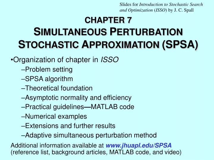
1. Slides for Introduction to Stochastic Search and Optimization (ISSO)by J. C. Spall CHAPTER 7 SIMULTANEOUS PERTURBATION STOCHASTICAPPROXIMATION(SPSA) Organization of chapter in ISSO Problem setting SPSA algorithm Theoretical foundation Asymptotic normality and efficiency Practical guidelines—MATLAB code Numerical examples Extensions and further results Adaptive simultaneous perturbation method Additional information available at www.jhuapl.edu/SPSA(reference list, background articles, MATLAB code, and video)

2. A. PROBLEM SETTING AND SPSA ALGORITHM • Consider standard minimization setting, i.e., find root  to where L() is scalar-valued loss function to be minimized and  is p-dimensional vector • Assume only (possibly noisy) measurements of L() available • No direct measurements of g() used, as are required in stochastic gradient methods • Noisy measurements of L() in areas such as Monte Carlo simulation, real-time control/estimation, etc. • Interested in p > 1 setting (including p >> 1)

3. SPSA Algorithm • Let () denote SP estimate of g() at kth iteration • Let denote estimate for  at kth iteration • SPSA algorithm has form where {ak} is nonnegative gain sequence • Generic iterative form above is standard in SA; stochastic analogue to steepest descent • Under conditions,  in “almost sure” (a.s.) stochastic sense as k

4. Computation of (•) (Heart of SPSA) • Let be vector of p independent random variables at kth iteration • typically generated by Monte Carlo • Let {ck} be sequence of positive scalars • For iteration kk+1, take measurements at design levels: where are measurement noise terms • Common special case is when (e.g., system identification with perfect measurements of the likelihood function)

5. Computation of (•) (cont’d) • The standard SP form for (•): • Note that(•) only requires two measurements of L(•) independentofp • Above SP form contrasts with standard finite-difference approximations taking 2p (or p+1) measurements • Intuitive reason why (•)is appropriate is that formalized in Section B

6. Essential Conditions for SPSA • To use SPSA, there are regularity conditions on L(), choice of k, the gain sequences {ak}, {ck}, and the measurement noise • Sections 7.3 and 7.4 of ISSO present essential conditions • Roughly speaking the conditions are: A. L() smoothness:L() is thrice differentiable function (can be relaxed—see Section 7.3 of ISSO) B. Choice of k distribution: For all k, k has independent components, symmetrically distributed around 0, and • Bounded inverse moments condition is critical (excludeski being normally or uniformly distributed) • Symmetric Bernoulli ki = 1 (prob = ½ for each outcome) is allowed; asymptotically optimal (see Section F or Section 7.7 of ISSO)

7. Essential Conditions for SPSA (cont’d) C. Gain sequences: standard SA conditions: (better to violate some of these gain conditions in certain practical problems; e.g., nonstationary tracking and control where ak = a > 0, ck = c > 0 k, i) D. Measurement Noise: Martingale difference k sufficiently large. (Noises not required to be independent of each other or of current/previous and k values.) Alternative condition (no martingale mean 0 assumption needed) is that be bounded k

8. Valid and Invalid Perturbation Distributions

9. B. THEORETICAL FOUNDATION Three Questions Question 1: Is (•) a valid estimator for g(•)? Answer:Yes, under modest conditions. Question 2:Will the algorithm converge to ? Answer:Yes, under reasonable conditions. Question 3:Do savings in data/iteration lead to a corresponding savings in converging to optimum? Answer:Yes, under reasonable conditions.

10. Near Unbiasedness of (•) • SPSA stochastic analogue to deterministic algorithms if is “on average” same as g(q) for any q • Suppressing iteration index k, mth component of (q) is: • With we have for any m:

11. Illustration of Near-Unbiasedness for (•) with p = 2 and Bernoulli Perturbations 7-11

12. Theoretical Basis (Sects. 7.3 – 7.4 of ISSO) • Under appropriate regularity conditions (e.g., thrice continuously differentiable, is martingale difference noise, etc.), we have: • Near Unbiasedness • Convergence: • Asymptotic Normality: where m, , and b depend on SA gains, k distribution, and shape of L()

13. Efficiency Analysis • Can use asymptotic normality to analyze relative efficiency of SPSA and FDSA (Spall, 1992; Sect. 7.4 of ISSO) • Analogous to SPSA asymptotic normality result, FDSA is also asymptotically normal (Chap. 6 of ISSO) The critical cost in comparing relative efficiency of SPSA and FDSA is number of loss function measurements y(•), not number of iterations per se • Loss function measurements represent main cost (by far)—other costs are trivial • Full efficiency story is fairly complex—see Sect. 7.4 of ISSO and references therein

14. Efficiency Analysis (cont’d) • Will compare SPSA and FDSA by looking at relative mean square error (MSE) of  estimate • Consider relative MSE for same no. of measurements, n(not same no. of iterations). Under regularity conditions above: () • Equivalently, to achieve same asymptotic MSE () • Results () and () are main theoretical results justifying SPSA

15. Paraphrase of ()above: • SPSA and FDSA converge in same number of iterations despite p-fold savings in cost/iteration for SPSA — or — • One properly generated simultaneous random change of all variables in a problem contains as much information for optimization as a full set of one-at-a-time changes of each variable

16. C. PRACTICAL GUIDELINES ANDMATLABCODE • The code below implements SPSA iterations k = 1,2,...,n • Initialization for program variables theta, alpha, etc. not shown since that can be handled in numerous ways (e.g., file read, direct inclusion, input during execution) • elements are generated by Bernoulli ±1 • Program calls external function loss to obtain y(q) values • Simple enhancements possible to increase algorithm stability and/or speed convergence • Check for simple constraint violation (shown at bottom of sample code) • Reject iteration if is too much greater than (requires extra loss measurement per iteration) • Reject iteration if is too large (does not require extra loss measurement)

17. Matlab Code for k=1:n ak=a/(k+A)^alpha; ck=c/k^gamma; delta=2*round(rand(p,1))-1; thetaplus=theta+ck*delta; thetaminus=theta-ck*delta; yplus=loss(thetaplus); yminus=loss(thetaminus); ghat=(yplus-yminus)./(2*ck*delta); theta=theta-ak*ghat; end theta If maximum and minimum values on elements of theta can be specified, say thetamax and thetamin, then two lines can be added below theta update line to impose constraints: theta=min(theta,thetamax); theta=max(theta,thetamin); 7-17

18. D.APPLICATION OFSPSA • Numerical Study: SPSA vs. FDSA • Consider problem of developing neural net controller (wastewater treatment plant where objectives are clean water and methane gas production) • Neural net is function approximator that takes current information about the state of system and produces control action • Lk() = tracking error, = neural net weights • Need to estimate  in real-time; used nondecaying ak =a, ck =c due to nonstationary dynamics • p = dim() = 412 • More information in Example 7.4 of ISSO

19. Wastewater Treatment System

20. RMS Error for Controllerin Wastewater Treatment Model 7- 20 0101600-Fig-8.3

21. E. EXTENSIONS AND FURTHER RESULTS • There are variations and enhancements to “standard” SPSA of Section A • Section 7.7 of ISSO discusses: (i) Enhanced convergence through gradient averaging/smoothing (ii) Constrained optimization (iii) Optimal choice of k distribution (iv) One-measurement form of SPSA (v) Global optimization (vi) Noncontinuous (discrete) optimization

22. (i) Gradient Averaging and Gradient Smoothing • These approaches may yield improved convergence in some cases • In gradient averaging is simply replaced by the average of several (say, q) SP gradient estimates • This approach uses 2q values of y(•) per iteration • Spall (1992) establishes theoretical conditions for when this is advantageous, i.e., when lower MSE compensates for greater per-iteration cost (2q vs. 2, q >1) • Essentially, beneficial in a high-noise environment (consistent with intuition!) • In gradient smoothing, gradient estimates averaged across iterations according to scheme that carefully balances past estimates with current estimate • Analogous to “momentum” in neural net/backpropagation literature

23. (ii) Constrained Optimization • Most practical problems involve constraints on  • Numerous possible ways to treat constraints (simple constraints discussed in Section C) • One approach based on projections (exploits well-known Kuhn-Tucker framework) • Projection approach keeps in valid region for all k by projecting into a region interior to the valid region • Desirable in real systems to keep (in addition to ) inside valid region to ensure physically achievable solution while iterating • Penalty functions are general approach that may be easier to use than projections • However, penalty functions require care for efficient implementation

24. (iii) Optimal Choice of k Distribution • Sections 7.3 and 7.4 of ISSO discuss sufficient conditions for k distribution (see also Sections A and B here) • These conditions guide user since user typically has full control over distribution • Uniform and normal distributions do not satisfy conditions • Asymptotic distribution theory shows that symmetric Bernoulli distribution is asymptotically optimal • Optimal in both an MSE and nearness-probability sense • Symmetric Bernoulli is trivial to generate by Monte Carlo • Symmetric Bernoulli seems optimal in many practical (finite-sample) problems • One exception mentioned in Section 7.7 of ISSO (robot control problem): segmented uniform distribution

25. (iv) One-Measurement SPSA • Standard SPSA use two loss function measurements/iteration • One-measurement SPSA based on gradient approximation: • As with two-measurement SPSA this form is unbiased estimate of to within • Theory shows standard two-measurement form generally preferable in terms of total measurements needed for effective convergence • However, in some settings, one-measurement form is preferable • One such setting: control problems with significant nonstationarities

26. (v) Global Optimization • SPSA has demonstrated significant effectiveness in global optimization where there may be multiple (local) minima • One approach is to inject Gaussian noise to right-hand side of standard SPSA recursion: where bk 0 and wk N(0,Ipp) • Injected noise wk generated by Monte Carlo • Eqn. (*) has theoretical basis for formal convergence (Section 8.4 of ISSO)

27. (v) Global Optimization (Cont’d) • Recent results show that bk= 0 is sufficient for global convergence in many cases (Section 8.4 of ISSO) • No injected noiseneeded for global convergence • Implies standard SPSA is global optimizer under appropriate conditions • Numerical demo on some tough global problems with many local minima yield global solution • Neither genetic algorithms nor simulated annealing able to find global minima in test suite • No guarantee of analogous relative behavior on other problems • Regularity conditions for global convergence of SPSA difficult to check

28. (vi) Noncontinuous (Discrete) Optimization • Basic SPSA framework for L() differentiable in  • Many important problems have elements in  taking only discrete (e.g., integer) values • There have been extensions to SPSA to allow for discrete  • Brief discussion in Section 7.7 of ISSO; see also references at SPSA Web site • SP estimate produces descent information although gradient not defined • Key issue in implementation is to control iterations and perturbations to ensure they are valid  values

29. F. ADAPTIVE SIMULTANEOUS PERTURBATION METHOD • Standard SPSA exhibits common “1st-order” behavior • Sharp initial decline • Slow convergence in final phase • Sensitivity to units/scaling for elements of  • “2nd-order” form of SPSA exists for speeding convergence, especially in final phase (analogous to Newton-Raphson) • Adaptive simultaneous perturbation (ASP) method (details in Section 7.8 of ISSO) • ASP based on adaptively estimating Hessian matrix • Addresses long-standing problem of finding “easy” method for Hessian estimation • Also has uses in nonoptimization applications (e.g., Fisher information matrix in Subsection 13.3.5 of ISSO)

30. Overview of ASP • ASP applies in either (i) Standard SPSA setting where only L() measurements are available (as considered earlier) (“2SPSA” algorithm) • or — (ii) Stochastic gradient (SG) setting where L() and g() measurements are available (“2SG” algorithm) • Advantages of 2nd-order approach • Potential for speedier convergence • Transform invariance (algorithm performance unaffected by relative magnitude of  elements) • Transform invariance is unique to 2nd-order algorithms • Allows for arbitrary scaling of  elements • Implies ASP automatically adjusts to chosen units for 

31. Cost of Implementation • For any p, the cost per iteration of ASP is Four loss measurements for 2SPSA  or  Three gradient measurements for 2SG • Above costs for ASP compare very favorably with previous methods: O(p2)loss measurements y(•) per iteration in FDSA setting (e.g., Fabian, 1971) O(p) gradient measurements per iteration in SG setting (e.g., Ruppert, 1985) • If gradient/Hessian averaging or y(•)-based iterate blocking is used, then additional measurements needed per iteration

32. Efficiency Analysis for ASP • Can use asymptotic normality of 2SPSA and 2SG to compare asymptotic RMS errors (as in basic SPSA) against best possible asymptotic RMS of SPSA and SG, say and • 2SPSA: With ak =1/k and ck = c/k1/6 (k 1) • 2SG: With ak = 1/k and any valid ck • Interpretation: 2SPSA (with ak = 1/k) does almost as well as unobtainable best SPSA; RMS error differs by < factor of 2 • 2SG (with ak = 1/k) does as well as the analytically optimal SG (rarely available)