Download
1 / 1
10 likes | 115 Views
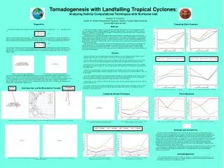
Study on helicity computational techniques post-Hurricane Ivan to analyze tornado environments in TCs, emphasizing helicity values and storm motion impacts.

E N D
Tornadogenesis with Landfalling Tropical Cyclones: Analyzing Helicity Computational Techniques with Hurricane Ivan Stephen R. Guimond Center for Ocean-Atmospheric Prediction Studies, Florida State University guimond@coaps.fsu.edu Comparing Storm Quadrant Diagnostics The vertically integrated helicity equation in a ground relative framework over a certain layer ( to ) can be expressed as: (1) where is the horizontal velocity vector and is the horizontal vorticity vector (Doswell 1991). In order to examine the amount of rotation from wind shear that individual storms may “feel” the storm relative helicity is computed by subtracting out the storm motion from the horizontal wind vector and inserting into equation (1). The horizontal vorticity vector is given by: (2) and can be broken down into streamwise (parallel to mean wind) and crosswise (perpendicular to mean wind) components (Doswell 1991). It is the streamwise vorticity component that is of most importance to studies of tornado environments as this parameter measures the amount of rotation along the wind that can be tilted into an upright vortex shown in the schematic diagrams below. Two variations for coding the calculation of both ground and storm relative helicity from soundings in Tallahassee (TLH) and Slidell (SIL) are used to examine the most physically appropriate method for hurricane-tornado environments. Version 1 involves using equations (1) and (2) directly in the helicity calculation while version 2 assumes that helicity is proportional to the area swept out by wind vectors for each coordinate frame (Fuelberg 2005;Leftwich 2005). In addition, variations in the determination of storm motion, calculated as a mass-weighted mean over a certain layer, are tested for each method and for varying helicity integration depths (McCaul 1991). Abstract A major source of property damage, injury and death with landfalling Tropical Cyclones (TCs) especially along the Gulf Coast are outbreaks of intense miniature supercells that frequently spawn tornadoes. Hurricane Ivan (2004) was a prime example of a landfalling TC that produced killer tornadoes associated with outer convective bands across the panhandle of Florida late on the 15th of September 2004. Tornado environments are typically diagnosed with parameters that measure the amount of vertical wind shear (both speed and directional) and buoyancy, two properties of the atmosphere that can produce rotating updrafts and mesocyclones. Helicity and streamwise vorticity, derived from the vertical wind shear, are main players in the formation of a tornadic vortex associated with energized supercell environments. Analysis of these parameters, as well as Convective Available Potential Energy (CAPE) and Convective INhibition (CIN), within TC environments can be complex due to the modulating influence of TCs on the large-scale flow. The present study attempts to examine the dynamic and thermodynamic parameters from above on the development of tornadic supercells in a TC environment with an emphasis on analyzing the skill of a program used to compute ground relative helicity (GRH) and storm relative helicity (SRH). Two versions will be examined including: (1) using the explicit mathematical derivation of helicity and (2) assuming helicity values are proportional to the area swept out by wind vectors in a certain layer of the atmosphere. Figure 3b. Time Series comparison of mean SRH for TLH. See key below. • Results • Figures 2a, 2b and 2c from TLH depict temporal evolution comparisons of each helicity calculation method for various integration depths along with storm cell motions from either 6 or 12 km layer mass weighted means. • Version 1 follows a pattern of helicity most reminiscent of tornado environments with a steady increase in storm relative values in the six hours or more before the tornado occurred in Blountstown and tapering off in the following 12 hours. • Peak values for this version reach 275 m2/s2 in the 0-2 km layer at 00 UTC and are attained with the 12 km cell motion, which appears to be close to a motion of ~30 to the right and 75% of the speed of the mean wind layer usually taken as 6 km (Leftwich 2005). • Version 2 from each plot appears to follow closely with version 1 until 00 UTC when values of storm relative helicity increase sharply while continuing to climb in the following 12 hours. Peak values for this version reach 450 m2/s2, with a 12 km cell motion. • Mean values of GRH and SRH for each integration depth for all comparisons were computed and are shown in Figures 3 and 4 for TLH and SIL, respectively. Mean helicity values from TLH are much larger than those from SIL, especially for SRH meaning that storms moving through the TLH region were able to “feel” more rotation. • From the plots, one can see that from 00 UTC and onward TLH was within the right front quadrant and SIL was within the left front quadrant of Ivan. • Also shown are the time series of CAPE and CIN for the same period in Figures 5 and 6, respectively. One can see the clear indication of the amount of buoyancy available to produce an upright vortex from the TLH soundings while SIL is hindered by a large amount of CIN. Figure 3a. Time Series comparison of mean GRH for TLH. See key below. Above: Schematic depicting how vertical wind shear can develop horizontal vorticity. Taken from WFO Little Rock. Above: Schematic of the generation of an upright vortex from a source of streamwise vorticity. Taken from Doswell 2000. Dry Air Intrusion Embedded Mini-Supercells Hurricane Ivan and the Blountstown Tornado Figure 4b. Time series comparison of mean SRH for SIL. See key above. Figure 4a. Time series comparison of mean GRH for SIL. See key above. Thermodynamics Comparing Helicity Techniques Left: MODIS visible image of Ivan on 15th Sept. 2004 (NASA) Center: Best track of Ivan (NHC) Right: GOES 3D visible enhancement of Ivan on 15th Sept. 2004 (NASA). Figure 1. Skew T-log p diagram with the closest spatial (~48 miles) and temporal (~2 hours) proximity to the Blountstown tornado. Figure 2a. Time series comparison of various methods for computing SRH in 0-2 km layer for TLH. See key below. Figure 6. Time series of CIN for TLH and SIL. See key below. Figure 5. Time series of CAPE for TLH and SIL. See key below. Summary and Conclusions An analysis of helicity computational techniques was presented, with hurricane Ivan as the guinea pig, in order to examine the most physically sound method of calculation. It was found that using the explicit equations depicted in (1) and (2) with a 12 km mass weighted cell motion provided for the best estimation of tornado potential for this particular TC. The 6 km layer motion used by McCaul 1991 produced helicity values that were somewhat small when compared to previous studies of TC-tornado environments. It is suggested that a 12 km cell motion incorporates the movement of right moving storms and deep convective clouds associated with mini-supercells in the outer bands of TCs. However, future testing with a 10 km cell motion may represent more realistic storm tops with SRH values that provide for a more physically consistent assessment of TC convective cells. In addition, time series of CAPE and CIN indicate that a significant amount of buoyancy was present in the soundings that can fuel strong rotating updrafts, something that was thought to be lacking in previous studies (McCaul 1991). Many of the time series plots of helicity, especially SRH, show indications of steadily increasing values within 6 or more hours of tornadogenesis. Knowledge of this type would prove useful to operational forecasters by heightening their awareness when watching for the threat of tornadoes with TCs although many more case studies are needed to determine anything concrete. Acknowledgements The author would like to thank Dr. Preston Leftwich for his expertise in calculating and interpreting helicity as well as for support throughout the entire process of this project. References and discussion pertaining to this project are available by e-mail directed to: guimond@coaps.fsu.edu Figure 2b. Time series comparison of various methods for computing SRH in 0-3 km layer for TLH. See key above. Figure 2c. Time series comparison of various methods for computing SRH in 0-6 km layer for TLH. See key above. Left: 0.5 base reflectivity from the TLH radar at 0208 UTC 16th September 2004. Right: 0.5 storm relative velocities from the TLH radar at 0208 UTC 16th September 2004 . Images courtesy of WFO TLH.