Download
1 / 21
210 likes | 336 Views
Lecture 16: Review. Mundell-Fleming AD-AS. Mundell-Fleming. e. IS : Y = C(Y-T) + I(Y,i) + G + NX(Y,Y*, E / (1+i-i*)). Interest parity. i. LM. IS. E. Y. e. E = E 1+i-i*. ------. * Fiscal and Monetary policy.

E N D
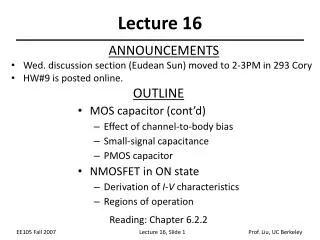
Lecture 16: Review • Mundell-Fleming • AD-AS
Mundell-Fleming e IS : Y = C(Y-T) + I(Y,i) + G + NX(Y,Y*, E / (1+i-i*)) Interest parity i LM IS E Y e E = E 1+i-i* ------ * Fiscal and Monetary policy
Fixed Exchange Rates (Credible) - A little bit of it even in “flexible” exchange rates systems; “commitment” to E rather than M => i = i* => M = YL(i*) P - Central Bank gives up monetary policy
Interest parity i LM i* IS E Y - Fiscal and Monetary policy - Capital controls; imperfect capital flows
Exchange Rate Crises i LM i* IS E Y Note: There is a shift in the IS as well… but this is small, especially in the short run
Building the Aggregate Supply • The labor market • Simple markup pricing • Long run (Natural rate: Aggregate demand factors don’t matter for Y) • Short run • Impact: Same as before but P also change (partial) • Dynamics (go toward Natural rate)
Wage Determination • Bargaining and efficiency wages e W = P F(u,z) Real wages Nominal wage setting Bargaining power Fear of unemployment Unemployment insurance Hiring rate (reallocation) Bargaining
Price Determination • Production function (simple) Y = N => P = (1+) W
The Natural Rate of Unemployment • “Long Run” P = P • The wage and price setting relationships: e W = F(u,z) P P = 1+ W => The natural rate of unemployment F(u,z) = 1 1+
W/P 1 1+ Price setting Wage setting u Unemployment n z, markup
From u to Y n n u = U = L - N = 1 - N = 1 - Y L L L L F(1 - Y /L, z) = 1 1+ n
W/P Wage setting 1 1+ Price setting Y Y n z, markup
Aggregate Supply e W = P F(1-Y/L,z) P = (1+ ) W => P = P (1+ ) F(1-Y/L,z) e
e P = P (1+ ) F(1-Y/L,z) AS P e P Y Y n
Aggregate Demand IS: Y = C(Y-T) + I(Y,i) + G LM: M = Y L(i) P LM’ [ P’ > P] i LM Y
AD:Y = Y(M/P, G, T) + + - P AD Y
AD-AS: Canonical Shocks AS P AD Yn Y Monetary expansion; fiscal expansion; oil shock
From AS to the Phillips Curve * The price level vs The inflation rate e P(t) = P (t) (1+ ) F(u(t), z) Note that: P(t)/P(t-1) = 1 + (P(t)-P(t-1))/P(t-1) P(t)/P(t-1) = 1 + (P(t)-P(t-1))/P(t-1) Let (t) = (P(t)-P(t-1))/P(t-1) e e
e (1+(t)) = (1+(t)) (1+ ) F(u(t), z) but ln(1+x) x if x is “small” Let also assume that ln(F(u(t), z)) = z – u(t) • Then
The Phillips Curve * The price level vs The inflation rate e P(t) = P (t) (1+ ) F(u(t), z) > (t) = (t) + (+z) - u(t) e
The Phillips Curve and The Natural Rate of Unemployment e (t) = (t) => u = (+z) (t) = (t) - (u(t) - u ) n e n