Figure 7 Measured equal loudness curves. 4

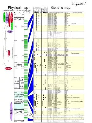
1. Modelling random changes in the parametersalong the length of the cochlea and the effect on hearing sensitivityEmery M. Ku1, Stephen J. Elliott1, Ben Lineton11ISVR, University of Southampton, UK Frequency [Hz] Figure 6 Inverse BM velocity of data presented in previous figure, now plotted against characteristic frequency. Variations in the micromechanical parameters of cochlear models can result in instability, which invalidates frequency-domain analysis. A general state space framework has been developed to determine the linear stability of cochlear models.3 Another benefit of the state space formulation is that it readily allows the model to be simulated in the time-domain. In order to produce an output pressure in the ear canal that can be compared with SOAE measurements, a two-port model of the middle and outer ears is incorporated into the model. The complete time-domain analysis involves three steps, which are illustrated below: 1) taking an input volume velocity in the ear canal, , to produce an output acceleration at the stapes, ; 2) this acceleration, , then becomes the input to a nonlinear time domain simulation of the cochlea that produces an output pressure at the round window, Pc(t); 3) Pc(t)is used to generate Pe(t), the output pressure in the ear canal that can be compared with SOAEs. Abstract The active cochlea is often modelled as having a uniformly varying distribution of parameters. In a real biological system, however, uniform distributions will always be disrupted by random spatial variations. In addition, noise-induced damage can be manifest as severe ‘focal lesions’ in the organ of Corti which compromise the cochlear amplifier in specific regions, thus also disturbing the smooth variation of parameters. A state space model of the cochlea has been developed that can be used to investigate the effect of such changes. The frequency responses of cochleae with near-unstable distributions of physical parameters are determined and compared with audiometric data. The limit cycles that are generated once the system does become unstable are then compared with measured spontaneous otoacoustic emissions. Linear, Stable Frequency Domain Results Introduction More than 8% of the population of many developed countries suffer from significant sensorineural hearing loss. In addition, approximately 90% of all hearing loss in adults is due to cochlear malfunction.1 This is a widespread problem that is only recently beginning to receive greater attention from scientists modelling cochlear mechanics. Most researchers agree upon the existence of a Cochlear Amplifier (CA) that actively enhances the response of the travelling wave as it propagates through the human cochlea. The CA is believed to be driven by the motility of the Outer Hair Cells (OHCs) in the organ of corti, though the exact mechanism by which the OHCs accomplish this is still a matter of debate. In this study, the micromechanical feedback gain in a discrete fluid-coupled cochlear model2, which is analogous to the activity of a local set of OHCs, is randomly perturbed as a function of position. Frequency-domain results are generated from a near-unstable linear system and compared with measured equal-loudness curves; time-domain results are also generated from an unstable nonlinear cochlea and compared with measured Spontaneous Otoacoustic Emissions (SOAEs). Figure 5 Basilar Membrane (BM) velocity responses given a near-unstable distribution of gains at several nominal gain levels. Figure 7 Measured equal loudness curves.4 Nonlinear, Unstable Time Domain Results These results were generated from a single unstable cochlea; the poles of this system are shown in Figure 8.b. A pulse was directly fed in to the simulation, (see Methods, 2). The spectrum of the output pressure in the cochlea was transformed to obtain the ear canal pressure (see Methods, 3), which is plotted in Figure 8.a. 20ms were simulated using MATLAB’s ode solver, ode45, given an output sampling rate of 100kHz. The spectra of the generated SOAEs are comparable to human measurements, such as the data shown in Figure 9. Methods Figure 9 Measured human SOAEs in one ear.5 Figure 8.a-b Response of an unstable nonlinear cochlea: a) pressure in the ear canal; b) detailed view of pole positions: the solid red line represents the boundary of stability, unstable poles are circled. 1) 2) Conclusions and Future Work The trends in the frequency domain analysis show good agreement with the equal loudness curves. Additionally, there is a regular spectral periodicity of the peaks in the frequency domain analysis, analogous to that observed in stimulus-frequency OAEs. This also occurs in the spacings of unstable poles, which agree with predictions.6 This will be the subject of a future publication. The SOAE spectrum obtained from the unstable cochlea shows good agreement with the stability analysis. However, distinct peaks at near-unstable frequencies and wider-than-expected bandwidths at unstable frequencies imply that transients are being included in the analysis. In order to cleanly resolve SOAEs, longer simulations are required. 3) Figure 4 Nonlinear, micromechanical model.3 Figures 1-4 Steps involved in the time-domain simulation of the nonlinear cochlea: from input volume velocity, Qe, to output ear canal pressure, Pe. References 1 Jesteadt, W. (Editor) (1997). Modeling Sensorineural Hearing Loss. Hillsdale, NJ: Erlbaum. 2 S.T. Neely, D.O. Kim, (1986). A model for active elements in cochlear biomechanics. J. Acoust. Soc. Am. 79(5) 3 S.J. Elliott, E.M. Ku, B. Lineton, (2007). A state space model for cochlear mechanics. Manuscript accepted for publication by J. Acoust. Soc. Am on 14th Aug, 2007. 4 Mauerman et al, (2004). Fine structure of the hearing threshold and loudness perception. J. Acoust. Soc. Am. 116 (1070) 5 Martin et al, (1990). Distortion product emissions in humans. I. Basic properties in normally hearing subjects., Ann Otol Rhinol Laryngol Suppl 147 (3-14). 6 G. Zweig and C.A. Shera, (1995). The origin of periodicity in the spectrum of emissions. J. Acoust. Soc. Am. 98 (4).