Download
1 / 45
780 likes | 1.9k Views
Chapter 2 : Formatting and Baseband Modulation. Contents. Formatting Sampling Theorem Pulse Code Modulation (PCM) Quantization Baseband Modulation. Introduction. Introduction. Formatting To insure that the message is compatible with digital signal

E N D
Contents • Formatting • Sampling Theorem • Pulse Code Modulation (PCM) • Quantization • Baseband Modulation
Introduction • Formatting • To insure that the message is compatible with digital signal • Sampling : Continuous time signal x(t) Discrete time pulse signal x[n] • Quantization : Continuous amplitude Discrete amplitude • Pulse coding : Map the quantized signal to binary digits • When data compression is employed in addition to formatting, the process is termed as a source coding. • Baseband Signaling: Pulse modulation • Convert binary digits to pulse waveforms • These waveforms can be transmitted over cable.
Formatting Textual Data (Cont.) • A system using a symbol set with a size of M is referred to as an M-ary system. • For k=1, the system is termed binary. • For k=2, the system is termed quaternary or 4-ary. M=2k • The value of k or M represents an important initial choice in the design of any digital communication system.
Formatting Analog Information • Baseband analog signal • Continuous waveform of which the spectrum extends from dc to some finite value (e.g. few MHz) • Analog waveform Sampled version • PAM Analog waveform FT Sampling process ((e.g.) sample-and-hold) Low pass filtering
Sampling Theorem • Uniform sampling theorem A bandlimited signal having no spectral components above fm hertz can be determined uniquely by values sampled at uniform intervals of
Nyquist Criterion • A theoretically sufficient condition to allow an analog signal to be reconstructed completely from a set of uniformly spaced discrete-time samples • Nyquist rate e.g.) speech 8kHz audio 44.1kHz
Impulse Sampling • In the time domain, • In the frequency domain,
Impulse Sampling (Cont.) FT FT FT
Impulse Sampling (Cont.) • The analog waveform can theoretically be completely recovered from the samples by the use of filtering (see next figure). • Aliasing If , some information will be lost. • Cf) Practical consideration • Perfectly bandlimited signals do not occur in nature. • A bandwidth can be determined beyond which the spectral components are attenuated to a level that is considered negligible.
Aliasing • Due to undersampling • Appear in the frequency band between
Sampling and aliasing • Helicopter 100Hz • Sampling at 220Hz 100Hz • Sampling at 80Hz 20Hz • How about sampling at 120Hz? -100 0 100 f -100 120 -320 340 0 100 f 320 -340 -120 540 -20 60 -100 -180 -140 -60 20 100 f
Aliasing (Cont.) • Effect in the time domain
Natural Sampling • More practical method • A replication of X(f), periodically repeated in frequency every fs Hz. • Weighted by the Fourier series coefficients of the pulse train, compared with a constant value in the impulse-sampled case.
Natural Sampling (Cont.) -1/T 1/T -1/T 1/T
Sample-and-Hold • The simplest and most popular sampling method • Significant attenuation of the higher-frequency spectral replicates • The effect of the nonuniform spectral gain P(f) applied to the desired baseband spectrum can be reduced by postfiltering operation.
Oversampling • the most economic solution • Analogprocessing is much more costly than digital one.
Quantization • Analog quantized pulse with “Quantization noise” • L-level uniform quantizer for a signal with a peak-to-peak range of Vpp= Vp-(-Vp) =2Vp • The quantization step • The sample value on is approximate to • The quantization error is o
Quantization Errors (Cont’d) • SNR due to quantization errors
Pulse Code Modulation (PCM) • Each quantization level is expressed as a codeword • L-level quantizer consists of L codewords • A codeword of L-level quantizer is represented by l-bit binary digits. • PCM • Encoding of each quantized sample into a digital word
PCM Word Size • How many bits shall we assign to each analog sample? • The choice of the number of levels, or bits per sample, depends on how much quantization distortion we are willing to tolerate with the PCM format. • The quantization distortion error p = 1/(2 # of levels)
Uniform Quantization • The steps are uniform in size. • The quantization noise is the same for all signal magnitudes. • SNR is worse for low-level signals than for high-level signals.
Nonuniform Quantization • For speech signals, many of the quantizing steps are rarely used. • Provide fine quantization to the weak signals and coarse quantization to the strong signals. • Improve the overall SNR by • The more frequent the more accurate • The less frequent the less accurate • But, we only have uniform quantizer. Probability Volt
Nonuniform Quantization (Cont.) • Companding = compress + expand • Achieved by first distorting the original signal with a logarithmic compression characteristic and then using a uniform quantizer. • At the receiver, an inverse compression characteristic, called expansion, is applied so that the overall transmission is not distorted. Probability Probability o o Volt Volt x[n] x[n]’ Compression Quantization Expansion
Baseband Transmission • Digits are just abstractions: a way to describe the message information. • Need something physical that will represent or carry the digits. • Represent the binary digits with electrical pulses in order to transmit them through a (baseband) channel. • Binary pulse modulation: PCM waveforms • Ex) RZ, NRZ, Phase-encoded, Multi-level binary • M-ary pulse modulation : M possible symbols • Ex) PAM, PPM (Pulse position modulation), PDM (pulse duration modulation)
PCM Waveform Types • Nonreturn-to-zero (NRZ) • NRZ-L, NRZ-M (differential encoding), NRZ-S • Return-to-zero (RZ) • Unipolar-RZ, bipolar-RZ, RZ-AMI • Phase encoded • bi--L (Manchester coding), bi--M, bi--S • Multilevel binary • Many binary waveforms use three levels, instead of two.
Choosing a PCM Waveform • DC component • Magnetic recording prefers no dc (Delay, Manchester..) • Self-clocking • Manchester • Error detection • Duobinary (dicode) • Bandwidth compression • Duobinary • Differential encoding • Noise immunity
Spectral Densities of PCM Waveforms • Normalized bandwidth • Can be expressed as W/RS [Hz/(symbol/s)] or WT • Describes how efficiently the transmission bandwidth is being utilized • Any waveform type that requires less than 1.0Hz for sending 1 symbol/s is relatively bandwidth efficient. • Bandwidth efficiency R/W [bits/s/Hz]
Spectral Densities of PCM Waveforms Bandwidth efficiency Mean = 0 DC=0 R/W [bits/s/Hz] Transition period↑ W ↓ FT
Autocorrelation of Bipolar Note that where xi+1 xi xi+2 xi-1 x(t) 0 To 2To xi xi+1 xi+2 xi-1 x(t+Ʈ) -Ʈ To-Ʈ 2To-Ʈ A2 A2 Rx(Ʈ) -Ʈ 0 To To-Ʈ 2To 2To-Ʈ
Autocorrelation of Bipolar Note that where xi+1 xi xi+2 xi-1 x(t) 2To 0 To xi xi+1 xi+2 xi-1 x(t+Ʈ) -Ʈ To-Ʈ 2To-Ʈ A2 A2 A2 Rx(Ʈ) -Ʈ 0 To To-Ʈ 2To 2To-Ʈ
Autocorrelation and power spectrum density of Bipolar Gx(f) 1 FT 0 0 0
M-ary Pulse-Modulation • M=2k-levels : k data bits per symbol longer transition period narrower W more channel • Kinds of M-ary pulse modulation • Pulse-amplitude modulation (PAM) • Pulse-position modulation (PPM) • Pulse-duration modulation (PDM) • M-ary versus Binary • Bandwidth and transmission delay tradeoff • Performance and complexity tradeoff
Example. Quantization Levels and Multilevel Signaling • Analog waveform fm=3kHz, 16-ary PAM, quantization distortion 1% (a) Minimum number of bits/sample? |e|= 1/2L < 0.01 L>50 L=64 6bits/sample (b) Minimum required sampling rate? fs > 2*3kHz = 6kHz (c) Symbol transmission rate? 9103symbols/sec 6*6 kbps = 36kbps 36[kbps]/4[bits/symbol] (d) If W=12kHz, the bandwidth efficiency? R/W = 36kbps / 12kHz = 3bps/Hz
HW#3 • P2.2 • P2.8 • P2.9 • P2.14 • P2.18