LOCO, Linear Optics from Closed Orbits
390 likes | 647 Views
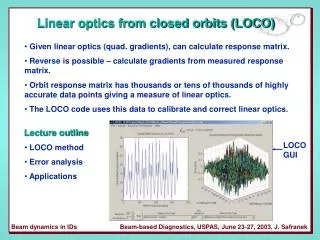
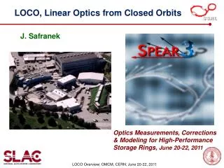
LOCO, Linear Optics from Closed Orbits. J. Safranek. Optics Measurements, Corrections & Modeling for High-Performance Storage Rings, June 20-22, 2011. Linear Optics from Closed Orbits (LOCO). Given linear optics (quad. gradients), can calculate response matrix.

LOCO, Linear Optics from Closed Orbits
E N D
Presentation Transcript
LOCO, Linear Optics from Closed Orbits J. Safranek Optics Measurements, Corrections & Modeling for High-Performance Storage Rings, June 20-22, 2011
Linear Optics from Closed Orbits (LOCO) • Given linear optics (quad. gradients), can calculate response matrix. • Reverse is possible – calculate gradients from measured response matrix. • Orbit response matrix has thousands or tens of thousands of highly accurate data points giving a measure of linear optics. • The LOCO code uses this data to calibrate and correct linear optics. • Lecture outline • LOCO method • Error analysis • Applications LOCO GUI
Development • W.J. Corbett, M.J. Lee, and V. Ziemann, “A fast model calibration procedure for storage rings,” SLAC-PUB-6111, May, 1993. • J. Safranek, “Experimental determination of storage ring optics using orbit response measurements”, Nucl. Inst. and Meth. A388, (1997), pg. 27. • G. Portmann et al., “MATLAB-based LOCO”, EPAC 2002. • X. Huang et al., “LOCO with constraints and improved fitting technique”, ICFA Beam Dynamics Newsletter, December, 2007. • This newsletter has several LOCO articles, and could serve as a LOCO tutorial. • The algorithm has been applied at many storage rings (and transport lines) worldwide. • JACoW search on LOCO keyword returns >200 hits, most of which are for orbit response matrix analysis.
LOCO Algorithm The orbit response matrix is defined as The parameters in a computer model of a storage ring are varied to minimize the c2 deviation between the model and measured orbit response matrices (Mmod and Mmeas). The si are the measured noise levels for the BPMs; E is the error vector. The c2 minimization is achieved by iteratively solving the linear equation For the changes in the model parameters, Kl, that minimize ||E||2=c2.
Response matrix review The response matrix is the shift in orbit at each BPM for a change in strength of each steering magnet. Vertical response matrix, BPM i, steererj: Horizontal response matrix: Additional h term keeps the path length constant (fixed RF frequency). LOCO option to use this linear form of the response matrix (faster) or can calculate response matrix including magnet nonlinearities and skew gradients (slower, more precise). First converge with linear response matrix, then use full response matrix.
Parameters varied to fit the orbit response matrix NSLS XRay Ring fit parameters: 56 quadrupole gradients 48 BPM gains, horizontal 48 BPM gains, vertical 90 steering magnet kicks =242 Total fit parameters NSLS XRay data: (48 BPMs)*(90 steering magnets) =4320 data points c2 fit becomes a minimization problem of a function of 242 variables. Fit converted to linear algebra problem, minimize ||E||2=c2. For larger rings, fit thousands of parameters to tens of thousands of data points. For APS, full matrix is ~9 Gbytes, so the size of the problem must be reduced by limiting the number of steering magnets in the response matrix. For rings the size of LHC, problem is likely too large to solve all at once on existing computers. Could divide ring into sections and analyze sections separately. Or consider alternative c2 minimization algorithm.
More fit parameters • Why add BPM gains and steering magnet calibrations? • Adding more fit parameters increases error bars on fit gradients due to propagation of random measurement noise on BPMs. If you knew that all the BPMs were perfectly calibrated, it would be better not to vary the BPM gains in the fit. • More fit parameters decreases error on fit gradients from systematic modeling errors. Not varying BPM gains introduces systematic error. • As a rule, vary parameters that introduce ‘significant’ systematic error. This usually includes BPM gains and steering magnet kicks. • Other parameters to vary: • Quadrupole roll (skew gradient) • Steering magnet roll • BPM coupling • Steering magnet energy shifts • Steering magnet longitudinal centers } Parameters for coupled response matrix,
Error bars from BPM measurement noise LOCO calculates the error bars on the fit parameters according to the measured noise levels of the BPMs. LOCO uses singular value decomposition (SVD) to invert and solve for fit parameters. The results from SVD are useful in calculating and understanding the error bars. SVD reduces the matrix to a sum of a product of eigenvectors of parameter changes, v, times eigenvectors, u, which give the changes in the error vector, E, corresponding to v. The singular values, wl, give a measure of how much a change of parameters in the direction of v in the multidimensional parameter space changes the error vector. (For a more detailed discussion see Numerical Recipes, Cambridge Press.)
SVD and error bars A small singular value, wl, means changes of fit parameters in the direction vl make very little change in the error vector. The measured data does not constrain the fit parameters well in the direction of vl; there is relatively large uncertainty in the fit parameters in the direction of vl. The uncertainty in fit parameter Kl is given by Illustration for 2 parameter fit: K2 Together the vl and wl pairs define an ellipse of variances and covariances in parameter space. LOCO converges to the center of the ellipse. Any model within the ellipse fits the data as well, within the BPM noise error bars. best fit model Ellipse around other models that also give good fit. K1
SVD and error bars, II Eigenvectors with small singular values indicate a direction in parameter space for which the measured data does not constrain well the fit parameters. The two small singular values in this example are associated with a degeneracy between fit BPM gains and steering magnet kicks. If all BPM gains are increased and kicks decreased by a single factor, the response matrix does not change. There two small singular values – horizontal and vertical plane. This problem can be eliminated by adding dispersion as a column of the response matrix. The measured orbit shift with RF frequency can be treated like another horizontal steering magnet, but with negligible error in kick size, because RF frequency is well calibrated. This calibrates absolute horizontal steerer kicks and BPM gains. Including coupling terms in the fit calibrates vertically gains and kicks. Singular value spectrum; green circles means included in fit; red X means excluded. 2 small singular values plot of 2 v with small w eigenvector, v BPM Gx BPM Gy qx qy energy shifts & K’s
Analyzing multiple data sets Analyzing multiple data sets provides a second method for investigating the variation in fit parameters from measurement noise. The results shown here are for the NSLS X-Ray ring, and are in agreement with the error bars calculated from analytical propagation of errors. N.B. Numerical simulations are also useful for determining accuracy of LOCO fits. For example, ATF simulations showed that BPM rolls can cause errors in skew gradient fits. (Panagiotidis, Wolski, PAC09)
Systematic error • The error in fit parameters from systematic differences between the model and real rings is difficult to quantify. • Typical sources of systematic error are: • Magnet model limitations – unknown multipoles; end field effects. • Errors in the longitudinal positions of BPMs and steering magnets. • Nonlinearities in BPMs. • electronic and mechanical • avoid by keeping kick size small. Fit dominated by systematics from BPM nonlinearity Fit dominated by BPM noise Increasing steering kick size
Systematic error, II Error vector histogram With no systematic errors, the fit should converge to Number of points (8640 total) N = # of data points M = # of fit parameters This plot shows results with simulated data with With real data the best fit I’ve had is fitting NSLS XRay ring data to 1.2 mm for 1.0 mm noise levels. Usually is considerably larger. The conclusion: In a system as complicated as an accelerator it is impossible to eliminate systematic errors. The error bars calculated by LOCO are only a lower bound. The real errors include systematics and are unknown. The results are still not useless, but they must be compared to independent measurements for confirmation.
LOCO fit for NSLS X-Ray Ring Before fit, measured and model response matrices agree to within ~20%. After fit, response matrices agree to 10-3. (Mmeas-Mmodel)rms = 1.17 mm
Confirming LOCO fit for X-Ray Ring LOCO predicts measured b’s, BPM roll. LOCO confirms known quadrupole changes, when response matrices are measured before and after changing optics.
Correcting X-Ray Ring hx LOCO predicts measured hx, and is used to findgradient changes that best restore design periodicity.
NSLS X-Ray Ring Beamsize The improved optics control in led to reduction in the measured electron beam size. The fit optics gave a good prediction of the measured emittances. The vertical emittance is with coupling correction off.
Adding constraints in LOCO (Xiaobiao Huang) • Constrained fitting to limit quadrupole gradient changes in fit. • Sometimes data is insufficient to fully constrain fit gradients • Reducing # of singular values gave unreliable results • Instead, add constraints to restrict magnitude of gradient changes: • Levenberg-Marquardt fitting algorithm • More robust convergence for LOCO fitting Gauss-Newton Gauss-Newton/steepest-descent, depending on l
Results from SOLEIL • Fit gradients w/out constraints (>6% corrections) • Fit gradients with contraints (<1.5% corrections) • Successfully corrected optics errors
Coupling & hy correction, LOCO Minimize hy and off-diagonal response matrix. Vary weight on hy column in fit. SPEAR 3 Lifetime, 19 mA, single bunch 4.5 hours Correction off Lifetime Coupling correction on 1.5 hours
Coupling correction at Australian Synchrotron • 28 skew quadrupoles • Well aligned machine • 55 mm y for sextupoles • 0.06% uncorrected coupling • 0.01% corrected coupling • Fit revealed girder alignment error • 1.3 pm confirmed by Touschek lifetime • Dowd et al., PRST-AB, 2011. Fit skew error finds mis-aligned girder Touschek lifetime confirms fit model ey.
Chromaticity Nonlinear x: (nx, ny) vs. frf agrees with model. Local chromaticity calibrated with LOCO shows no sextupole errors:
Conclusion • LOCO has successfully corrected the optics of many storage rings, and some transport lines. It is a powerful algorithm for: • finding and correcting BPM and steering magnet errors, • finding and correcting normal and skew gradient errors, • correcting b and h, • correcting for ID focusing, • minimizing coupling, • calibrating transverse impedance and chromatic errors. • I look forward to further developments.
Different goals when applying LOCO • There are a variety of results that can be achieved with LOCO: • Finding actual gradient errors. • Finding changes in gradients to correct betas. • Finding changes in gradients to correct betas and dispersion. • Finding changes in local gradients to correct ID focusing. • Finding changes in skew gradients to correct coupling and hy. • Finding transverse impedance. The details of how to set up LOCO and the way the response matrix is measured differs depending on the goal.
LOCO GUI fitting options menu Remove bad BPMs or steerers from fit. Include coupling terms (Mxy, Myx) Model response matrix: linear or full non-linear; fixed-momentum or fixed-path-length Include h as extra column of M Let program choose Ds when calculating numerical derivatives of M with quadrupole gradients. Reject small singular values Optimize numerical accuracy Reject outlier data points
Finding gradient errors at ALS • LOCO fit indicated gradient errors in ALS QD magnets making by distortion. • Gradient errors subsequently confirmed with current measurements. • LOCO used to fix by periodicity. • Operational improvement (Thursday lecture).
SVD and error bars, III LOCO throws out the small singular values when inverting and when calculating error bars. This results in small error bars calculated for BPM gains and steering magnet kicks. The error bars should be interpreted as the error in the relative gain of one BPM compared to the next. The error in absolute gain is much greater. If other small singular values arise in a fit, they need to be understood. small error bars vertical BPM gain vertical BPM number
Fitting energy shifts. Horizontal response matrix: Betatron amplitudes and phases depend only on storage ring gradients: Dispersion depends both on gradients and dipole field distribution: If the goal is to find the gradient errors, then fitting the full response matrix, including the term with h, will be subject to systematic errors associated with dipole errors in the real ring not included in the model. This problem can be circumvented by using a “fixed momentum” model, and adding a term to the model proportional to the measured dispersion is a fit parameter for each steering magnet. In this way the hmodel is eliminated from the fit, along with systematic error from differences between hmodel and hmeas.
Correcting betas in PEPII Often times, finding the quad changes required to correct the optics is easier than finding the exact source of all the gradient errors. For example, in PEPII there are not enough BPMs to constrain a fit for each individual quadrupole gradient. The optics still could be corrected by fitting quadrupole families. Independent bmeasurements confirmed that LOCO had found the real b’s(x2.5 error!) Quadrupole current changes according to fit gradients restored ring optics to the design. PEPII HER by,design PEPII HER by,LOCO fit
Finding gradient errors • If possible, measure two response matrices – one with sextupoles off and one with sextupoles on. • Fit the first to find individual quadrupole gradients. • Fit the second to find gradients in sextupoles. • Fewer gradients are fit to each response matrix, increasing the accuracy. • … Measure a 3rd response matrix with IDs closed. • Vary all quadrupole gradients individually (maybe leave dipole gradient as a family). • Use either 1.) fixed-momentum response matrix and fit energy shifts or 2.) fixed-path-length depending on how well 1/r in the model agrees with 1/r in the ring (i.e. how well is the orbit known and controlled). • Get the model parameters to agree as best as possible with the real ring: model dipole field roll-off; check longitudinal positions of BPMs and steering magnets; compensate for known nonlinearities in BPMs. • Add more fitting parameters if necessary to reduce systematic error (for example, fit steering magnet longitudinal centers in X-Ray Ring.)
Correcting betas and dispersion • Measure response matrix with ring in configuration for delivered beam. • Sextupoles on • Correct to golden orbit • IDs closed (depending on how you want to deal with ID focusing) • Fit only gradients that can be adjusted in real ring. • Do not fit gradients in sextupoles or ID gradients • If a family of quadrupoles is in a string with a single power supply, constrain the gradients of the family to be the same. • To correct betas only, use fixed-momentum model matrix and fit energy shifts, so dispersion is excluded from fit. • To correct betas and dispersion, use fixed-path length matrix and can use option of including h as an additional column in response matrix. • To implement correction, change quadrupole current of nthquadrupole or quad family:
Insertion device linear optics correction • The code LOCO can be used in a beam-based algorithm for correcting the linear optics distortion from IDs with the following procedure: • Measure the response matrix with the ID gap open. • Then the response matrix is measured with the gap closed. • Fit the first response matrix to find a model of the optics without the ID distortion. • Starting from this model, LOCO is used to fit a model of the optics including the ID. In this second fit, only a select set of quadrupoles in the vicinity of the ID are varied. The change in the quadrupole gradients between the 1rst and 2nd fit models gives a good correction for the ID optics distortion. • Alternatively, LOCO can be used to accurately fit the gradient perturbation from the ID, and the best correction can be calculated in an optics modeling code. • This algorithm also works for ID coupling correction.
Linear optics correction at ALS Before correction Beta function distortion from wiggler. At ALS the quadrupoles closest to the IDs are not at the proper phase to correct optics distortions, so the optics correction cannot be made entirely local. Quadrupole changes used for correction After correction D. Robin et al. PAC97
Skew quadrupole compensation for ALS EPUs • Beamsize variation was solved in 2004: Installed correction coils for feedforward based compensation – routine use since June/September • Early 2005 we identified the root cause: 2-3 micron correlated motion of magnet modules due to magnetic forces • Will be able to modify design of future device such that active correction will not be necessary! C. Steier • Just for reference: Whenever an undulator moves, about 120-150 magnets are changed to compensate for the effect (slow+fast feed-forward, slow+fast feedback)