Download
1 / 44
440 likes | 573 Views
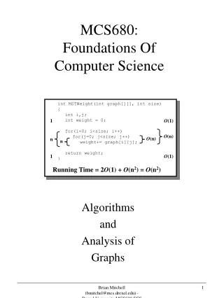
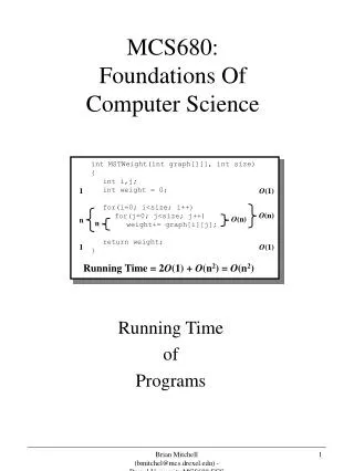
int MSTWeight(int graph[][], int size) { int i,j; int weight = 0; for(i=0; i<size; i++) for(j=0; j<size; j++) weight+= graph[i][j]; return weight; }. 1 1. O (1) O (1). O (n). O (n). n. n. Running Time = 2 O (1) + O (n 2 ) = O (n 2 ).

E N D
int MSTWeight(int graph[][], int size) { int i,j; int weight = 0; for(i=0; i<size; i++) for(j=0; j<size; j++) weight+= graph[i][j]; return weight; } 1 1 O(1) O(1) O(n) O(n) n n Running Time = 2O(1) + O(n2) = O(n2) MCS680:Foundations Of Computer Science Running Time of Programs Brian Mitchell (bmitchel@mcs.drexel.edu) - Drexel University MCS680-FCS
Introduction • Choosing an algorithm • Simplicity • Easy to code • Minimize code defects (bugs) • Generally tradeoff “easy-to-implement” for slower performance • Good for small or controlled input sizes • Selection Sort versus Merge Sort • Clarity • Algorithms should be clear and well-documented • Simplifies software maintenance issues • Efficiency • Generally efficient algorithms are harder to understand and implement • Efficient algorithms are required when: • We are concerned about running time • Generally a function of input size • We are concerned about runtime resources • Memory, bandwidth, processor capacity Brian Mitchell (bmitchel@mcs.drexel.edu) - Drexel University MCS680-FCS
Measuring Running Time • Approaches • Benchmarking • Develop representative input samples • Execute algorithm against input samples • Measure performance (Execution Time) • Must be careful of algorithm anomalies • Some algorithms performance is a direct function of the input data and not the size of the input data • Analysis • Group inputs according to size • The number of elements to be sorted, the number of nodes or edges in a graph, etc. • Determine a function, T(n), to model the number of units of time taken by an algorithm on any input size, n. • Because some algorithms performance is affected by the particular input sequence we should consider • Worst Case and Average Case running times Brian Mitchell (bmitchel@mcs.drexel.edu) - Drexel University MCS680-FCS
Running Time Example -Inner Loop of Selection Sort Consider the following code fragment: • Assignment of small to i takes 1 time unit • Assignment of j=(i+1) takes 1 time unit • Consider the if statement: • Comparison takes 1 time unit • Assignment of j to small takes 1 time unit • Worst case is that the comparison and assignment operation happens on every loop iteration • Thus, the if statement takes 2 time units • Consider the for loop • Loop is executed (n-i) times • Each time j is compared to n and incremented • Total of 2 time units per loop iteration small = i; for (j=(i+1); j<n; j++) if(A[j] < A[small]) small = j; Brian Mitchell (bmitchel@mcs.drexel.edu) - Drexel University MCS680-FCS
Running Time Example -Inner Loop of Selection Sort Consider the following code fragment: • Total Running Time • Loop Execution Time: • Body (if statement) is 2 units • Loop is executed (n-i) times • Loop management takes 2 units per iteration • Total loop time is 4(n-i) • Initialization/Termination Time: • 1 unit for assigning small from i • 1 unit for initializing j (to i+1) • 1 additional unit for the last (j<n) comparison • Happens when j=n (last time around the loop) • Total Running Time • T(n) = 4(n-i) + 3, letting m=(n-i+1) we get: • T(m) = 4m -1 (Linear Growth!) small = i; for (j=(i+1); j<n; j++) if(A[j] < A[small]) small = j; Brian Mitchell (bmitchel@mcs.drexel.edu) - Drexel University MCS680-FCS
Approximate Running Time-“Big-Oh” • Running Time Factors • The computer running the algorithm • CPU, Architecture, Bus, ... • The compiler used to generate the machine code • Some compilers generate better code that others • Prevents us from determining the actual running time of the program • Approximate Running Time • Use “Big-Oh” notation • Use of “Big-Oh” abstracts • Average machine instructions generated by the compiler • The number of machine instructions executed per second on a given computer • Promotes a “level playing field” for comparing algorithm running times Brian Mitchell (bmitchel@mcs.drexel.edu) - Drexel University MCS680-FCS
Simplifying Analysis With“Big-Oh” • In a previous example we estimated the running time of the inner loop of the Selection Sort. • T(m) = 4m - 1 • However we made some assumptions that are probably not true • All assignments take the same amount of time • A comparison takes the same amount of time as an assignment • A more accurate assessment would be: • The running time of the inner loop of the Selection Sort is some constant times m plus or minus another constant • T(m) = am + b where {a,b} are unknown constants • Estimate with Big-Oh: • Running time of inner loop of selection sort is O(m). Brian Mitchell (bmitchel@mcs.drexel.edu) - Drexel University MCS680-FCS
Definition-Big-Oh • Consider O(f(m)) • Definition of O(f(m)) is: • The worst case running time is some constant times f(m) • Examples • O(1) = some constant times 1 • O(m) = some constant times m • O(m2) = some constant times m2 • O(lg m) = some constant times lg m • Because a constant is built into the Big-Oh notation we can eliminate any constants from our runtime analysis, thus • T(m) = 4m - 1 = O(4m - 1) • O(4m - 1) = O(4m) + O(1) • But because Big-Oh notation has a constant built in: • O(4m) + O(1) = O(m) + O(1) but O(1) is a constant and constants are built in to Big-Oh • O(4m - 1) = O(m) Brian Mitchell (bmitchel@mcs.drexel.edu) - Drexel University MCS680-FCS
Big-OhNotation • In the previous slide we claimed thatO(4m - 1) is O(m) • Recall that Big-Oh notation is a worst case upper bound on execution complexity • We can prove that O(4m-1) is O(m) if we can find a constant, c, that holds for • (4m - 1) <= cm for all m>= 0 • Hence if c=4 then (4m-1) <= 4m for all m>=0 • Thus O(4m-1) is O(4m) • Because Big-Oh notation has a constant built into the definition we can show that O(4m) is O(m) • Suppose that O(4m) = O(m) • For O(4m) choose the implicit constant to be 1 • For O(m) choose the implicit constant to be 4 • Thus because of the implicit constant we know that O(4m) is O(m) • Thus we showed by manipulating the internal constant that O(4m-1) is O(4m) which is O(m) Brian Mitchell (bmitchel@mcs.drexel.edu) - Drexel University MCS680-FCS
Simplifying Big-OhExpressions • Remember: • Big-Oh expressions infer a built-in constant • Big-Oh expressions are a worst-case upper bound for execution complexity • Simplification Rules • Constant Factors Do Not Matter! • Because Big-Oh expressions implicitly contain a constant, you may drop the explicit constant • O(10000m) is O(m) implicit constant is 10000 • Low Order Terms Do Not Matter! • Remember that Big-Oh is an upper bound! • If T(n) = aknk+ak-1nk-1+...+a2n2+a1n+a0 thenT(n) [ak + ak-1 + ... + a2 + a1 + a0]nk • Thus T(n) is O([ak + ak-1 + ... + a2 + a1 + a0]nk) • If we let c = [ak + ak-1 + ... + a2 + a1 + a0] then c is a constant • Thus T(n) is O(c•nk) • Thus T(n) is O(nk) because constant factors do not matter Brian Mitchell (bmitchel@mcs.drexel.edu) - Drexel University MCS680-FCS
Simplifying Big-Oh Expressions: An Example • Suppose that we have a programs whose running time is T(0)=1, T(1)=4, T(2)=9, and in general T(n) = (n+1)2: • Thus T(n) = n2 + 2n + 1 • Because we are interested in an upper bound we can state that: • T(n) n2 + 2n2 + 1n2 • Thus T(n) 4n2 for all n > 0 because a polynomial expression is always less then the sum of the polynomial coefficients taken to the power of the highest power of n • This demonstrates the rule that low order terms do not matter • Thus T(n) is O(4n2) • But recall the rule that constant factors do not matter • Thus T(n) is O(n2) Brian Mitchell (bmitchel@mcs.drexel.edu) - Drexel University MCS680-FCS
Simplifying Big-Oh Expressions: An Example Brian Mitchell (bmitchel@mcs.drexel.edu) - Drexel University MCS680-FCS
Simplifying Big-Oh Expressions • We just saw two mechanisms for simplifying Big-Oh expressions • Dropping constant factors • Dropping low order terms • These rules will greatly simplify our analysis of “real” programs and algorithms • Other Rules • Big-Oh expressions are transitive • Recall that transitivity means that if A B and B C then A C • The relationship “is of Big-Oh” is another form of transitivity • If f(n) is O(g(n)) and O(g(n)) is O(h(n)) then it follows by transitivity that f(n) is O(h(n)) • Proof: Let c1 and c2 be constants. Therefore, f(n) c1•g(n) and g(n) c2•h(n). Thus,f(n) c1c2 •h(n) by transitivity. But c1c2 is a constant resulting in f(n) being of O(h(n)) Brian Mitchell (bmitchel@mcs.drexel.edu) - Drexel University MCS680-FCS
Tightness of Big-OhExpressions • Goal: we want the “tightest” big-oh upper bound that we can prove • Because big-oh is an upper bound we can imply that: • O(n) is O(n2) or O(n3) • Conversely, O(n3) is not O(n2) or O(n) • In general O(nk) • IS O(nx) for x k • But it IS NOT O(nz) for z < k • The following table lists some of the more common running times for programs and their informal names: Brian Mitchell (bmitchel@mcs.drexel.edu) - Drexel University MCS680-FCS
Consider the following function that returns TRUE if the input number is a power of 2 Analysis The while loop is executed until x reaches 1 or until x becomes an odd value Thus we execute the loop by dividing n by 2 a maximum of k times for n = 2k Taking the log of both sides we get log2 n = k which is lg n Thus PowerOfTwo() is O(lg n) Logarithms in Big-Oh Analysis #define ODD(x) ((x%2) == 1) BOOL PowerOfTwo(unsigned int x) { if (x == 0) return FALSE; while (x > 1) if(ODD(x)) return FALSE; else x /= 2; return TRUE; } Brian Mitchell (bmitchel@mcs.drexel.edu) - Drexel University MCS680-FCS
PowerOfTwo()Execution Complexity • Notice how T(n) is bounded by O(lg n) Brian Mitchell (bmitchel@mcs.drexel.edu) - Drexel University MCS680-FCS
Summation Rule For Big-Oh Expressions • Technique for summing Big-Oh expressions • As shown before we can drop constants and lower-order terms when analyzing running times • Same rule applies to summing Big-Oh expressions • Also recall that Big-Oh expressions are an upper bound • O(n) is O(n2) • O(lg n) is O(n) • RULE: Given O(f(n)) + O(g(n)) take the part with the larger complexity and drop the other part • O(n) + O(n2) = O(n2) • O(lg n) + O(n) = O(lg n) • O(1) + O(n) = O(n) Brian Mitchell (bmitchel@mcs.drexel.edu) - Drexel University MCS680-FCS
Example: Summation of Big-Oh Expressions • Consider the following algorithm that places 1’s in the diagonal of a matrix void DiagonalOnes(int A[][], int n) { int i,j; for(i = 0; i < n; i++) for(j = 0; j < n; j++) A[i][j] = 0; for(i = 0; i < n; i++) A[i][i] = 1; } O(n2) O(n) • Analysis • The zeroing phase of the algorithm takes two loops to initialize all matrix elements to zero • Both loops are bounded [0...n], this is O(n2) • The diagionalization phase of the algorithm requires one loop to place 1’s on the matrix diagional • Loop is bounded [0...n], this is O(n) • Total execution time is O(n2) + O(n) = O(n2) Brian Mitchell (bmitchel@mcs.drexel.edu) - Drexel University MCS680-FCS
Analyzing the Running Time of a Program • Goal: Develop techniques for analyzing algorithms and programs • Simple and tight bounds on execution complexity • Break the program or algorithm up into individual parts • Simple statements • Loops • Conditional statements • Procedure/Function calls • Analyze the individual parts in context to develop a Big-Oh expression • Simplify the Big-Oh expression Brian Mitchell (bmitchel@mcs.drexel.edu) - Drexel University MCS680-FCS
Simple Statements • All simple statements take O(1) time unless the statement is a function call • O(1) time indicates that a constant amount of time is required to execute the statement • Simple statements are: • Arithmetic expressions • z = a + b; • Input/Output (file, terminal, network) • gets(name); • printf(“%s\n”,”Hello World!”); • Array or structure accessing statements • a[1][2] = 9; • customer.age = 30; • linkedListPtr = linkedListPtr->next; Brian Mitchell (bmitchel@mcs.drexel.edu) - Drexel University MCS680-FCS
Analyzing For Loops • For loops are syntactically developed to specify the lower bound, the upper bound and the increment of the looping construct • for(i = 0; i < n; i++) • Given a for loop it is easy to develop an upper bound for the number of times that the loop will be executed • Can always leave the loop early with a goto, return or break statement • Goal: Determine an upper bound on the number of times that loop body will be executed • Analysis: Upper bound on the execution of a for loop is • (number of times loop is executed) * (execution time for body of the loop) +O(1) for initializing the loop index +O(1) for the last comparison Brian Mitchell (bmitchel@mcs.drexel.edu) - Drexel University MCS680-FCS
Analyzing Conditional Statements • Conditional statements typically takes the form: • if <condition> then <if-part>else <else-part> • Execution a conditional statement involves • A condition to test • An if-part that is executed if the condition is TRUE • An optional else-part that is executed if the condition is FALSE • Condition part takes O(1) unless it involves a function call • Let the if-part take O(f(n)) • Let the else-part (if present) take O(g(n)) • Thus • If the else-part is missing, running time is O(f(n)) • If the else-part is present, running time is O(max(f(n),g(n))) Brian Mitchell (bmitchel@mcs.drexel.edu) - Drexel University MCS680-FCS
Running Time Example:Simple, Loop and Conditionals • Consider the following code fragment if(A[0][0] = 0) for(i = 0; i < n; i++) for(j = 0; j < n; j++) A[i][j] = 0; else for(i = 0; i < n; i++) A[i][j] = 1; O(n2) O(n) O(1) O(n) O(1) • Analysis • Running time of the if-part [f(n)] is O(n2) • Running time of the else-part [g(n)] is O(n) • Total execution time is O(max(f(n),g(n))) which is O(max(n2,n)) • Thus total execution time is O(n2) Brian Mitchell (bmitchel@mcs.drexel.edu) - Drexel University MCS680-FCS
Analyzing Blocks • A block of code consists of a sequence of one or more statements • begin...end in Pascal • {...} in C, C++ and Java • Statements in a block may be • Simple statements • Complex statements (for, while, if,...) • Total execution time is the sum of all of the statements in the block • Use techniques (rule of sums) to simplify the expression • Thus if a block contains n statements, the execution time is: Brian Mitchell (bmitchel@mcs.drexel.edu) - Drexel University MCS680-FCS
Analyzing While and RepeatLoops • There is no (implicit) upper limit on the number of times that a while or repeat loop is executed • Analysis must determine an upper bound on the number of times that the loop is executed • Execution complexity is the number of times around the loop multiplied by the execution complexity of the loop body • The following code fragment can be shown to be O(n) BOOL FindIt(int A[], int n) { int i = 0; while((A[i] != val)&&(i < n)) i++; return (i != n) } Brian Mitchell (bmitchel@mcs.drexel.edu) - Drexel University MCS680-FCS
Using Trees to Model Analysis of Source Code Fragments • Technique: Build tree and develop execution complexity by traversing the tree from the bottom up to the tree root (1) for(i=0; i<(n-2); i++) { (2) small = i; (3) for(j=i+1; j<n; j++) (4) if(A[j] < A[small]) (5) small = j; (6) temp = A[small]; (7) A[small] = A[i]; (8) A[i] = temp; } for [1-8] block [2-8] [2] for [3-5] [6] [7] [8] if [4-5] [2] Brian Mitchell (bmitchel@mcs.drexel.edu) - Drexel University MCS680-FCS
Analyzing Procedure Calls • Task for analyzing code with procedure calls involves • Treating the procedure call as a simple statement • Use O(f(n)) is place of O(1) for the procedure call where f(n) is the execution complexity of the actual procedure call • Must fully analyze the procedure call prior to evaluating it in context • If the procedure is a recursive call then it must be analyzed by using other techniques • Generally the execution complexity can be modeled by performing an inductive proof on the number of times that the recursive call is performed • See the previous analysis of the Factorial() function Brian Mitchell (bmitchel@mcs.drexel.edu) - Drexel University MCS680-FCS
Analyzing Recursive Procedure Calls • Analyzing recursive procedure calls is more difficult then analyzing standard procedure calls • Technique: To analyze a recursive procedure call we must associate with each procedure P an unknown running time Tp(n) that defines P’s running time as a function of n • Must develop a recurrence relation • Tp(n) is normally developed by an induction on the size of argument n • Must set up the recurrence relation in a way that ensures that the size of the argument n decreases as the recurrence proceeds • The recurrence relation must specify 2 cases • The argument size is sufficiently small that no recursive calls will be made by P • The argument size is sufficiently large that recursive calls will be made Brian Mitchell (bmitchel@mcs.drexel.edu) - Drexel University MCS680-FCS
Recursive Call Analysis -Technique • To develop Tp(n) we examine the procedure P and do the following: • Use the techniques that we already developed to analyze P’s non-recursive call statements • Let Tp(n) be the running time of the recursive calls in P • Now reevaluate P twice: • Develop the base case. Evaluate P on the assumption that n is sufficiently small that no recursive procedure calls are made • Develop the inductive definition. Evaluate P on the assumption that n is large enough to result in recursive calls being made to P • Replace big-oh terms such as O(f(n)) by a constant times the function involved • O(f(n)) cf(n) • Solve the resultant recurrence relation Brian Mitchell (bmitchel@mcs.drexel.edu) - Drexel University MCS680-FCS
Recursive Call Analysis Example - Factorial • Consider the following code fragment int Factorial(int n) { (1) if (n <= 1) (2) return 1; else (3) return n * Factorial(n-1); } • Analysis • Determination of a good recursive procedure • There is a basis case (n <= 1) • There is an inductive case for n > 1 • For the basis case (n <= 1) • Lines (1) and (2) are executed, each are O(1), thus the total execution time for the base case is O(1) • For the inductive case (n > 1) • Lines (1) and (3) are executed, line (1) is O(1) and line (3) is O(1) for the multiplication and T(n-1) for the recursive call • Thus total time for the inductive case is:O(1) + T(n-1) Brian Mitchell (bmitchel@mcs.drexel.edu) - Drexel University MCS680-FCS
Recursive Call Analysis Example - Factorial • Analysis (con’t) • Thus the running time of Factorial() can be modeled by the following recurrence relation • Basis: T(1) = O(1) • Inductive: T(n) = O(1) + T(n-1) • Now replace big-oh expressions by constants • Basis: T(1) = a • Inductive: T(n) = b + T(n-1), for n > 1 • Now solving the recurrence relation • T(1) = a • T(2) = b + T(1) = a + b • T(3) = b + T(2) = a + 2b • In general, T(n) = a + (n-1)b for all n>1 • T(n) = a + (n-1)b = a + bn - b = (a-b) + bn • Thus T(n) = bn + (a-b), but (a-b) is a constant • The result is T(n) = bn + c (where c = (a-b)) • In big-oh terms T(n) is O(n) + O(1) = O(n) • Thus, Factorial() is O(n) Brian Mitchell (bmitchel@mcs.drexel.edu) - Drexel University MCS680-FCS
Analysis of MergeSort void MergeSort(mList list) { mList SecondList; if (list != NULL) { if(list->next != NULL) { SecondList = Split(list); MergeSort(list); MergeSort(SecondList); list = Merge(list,SecondList); } } } • Analysis of MergeSort() • Must determine the running time of • Split() and Merge() • Use the recursive technique to analyze MergeSort() Brian Mitchell (bmitchel@mcs.drexel.edu) - Drexel University MCS680-FCS
Analysis of Split() mList Split(mList orig) { mList secondCell; if (orig == NULL) return NULL; else if (orig->next == NULL) return NULL; else { secondCell = orig->next; orig->next = secondCell->next; secondCell->next = Split(secondCell->next); return secondCell; } } • Analysis of Split() • Basis Case: O(1) + O(1) = O(1) • Basis case is for n=0 and n=1 (two if statements) • Inductive Case: O(1)+O(1)+T(n-2)+O(1) • This is O(1) + T(n-2) BASIS INDUCTIVE Brian Mitchell (bmitchel@mcs.drexel.edu) - Drexel University MCS680-FCS
Analysis of Split() • Analysis of Split (Con’t) • Replace big-oh expressions by constants • BASIS CASE (n = {0,1}): • List is empty, first if statement is executed • List length is zero T(0) = a • List contains 1 element, first and second if statement is executed • List length is one T(1) = b • INDUCTIVE CASE (n > 1): • T(n) = O(1) + T(n-2) • T(n) = c + T(n-2) • T(2) = c + T(0) = a + c • T(3) = c + T(1) = b + c • T(4) = c + T(2) = a + 2c • T(5) = c + T(3) = b + 2c • In general for EVEN n, T(n) = a + cn/2 • In general for ODD n, T(n) = b + c(n-1)/2 • For any input list, the size of the list must be EVEN or ODD Brian Mitchell (bmitchel@mcs.drexel.edu) - Drexel University MCS680-FCS
Analysis Of Split() • Because any input list to Split() must be even or odd, the worst case running time is the maximum time that it takes to process an even or an odd sized input list • Even Sized List: • T(n) = a + cn/2, let constant m = c/2 • Thus T(n) = a + m(n/2) • Thus T(n) = O(1) + O(n) = O(n) • Odd Sized List: • T(n) = b + c(n-1)/2 = b + cn/2 - c/2 • Let constant m = c/2 • Thus T(n) = (b-m) + m(n/2) • Let constant p = (b-m) • T(n) = p + m(n/2) • Thus T(n) = O(1) + O(n) = O(n) • Thus split is O(n) because both odd and even sized lists are O(n) Brian Mitchell (bmitchel@mcs.drexel.edu) - Drexel University MCS680-FCS
Analysis of Merge() mList Merge(mList lst1, mList lst2) { mList *ml; if (lst1 == NULL) ml = lst2; else if (lst2 == NULL) ml = lst1; else if (lst1->element <= lst2->element) { lst1->next = Merge(lst1->next, lst2); ml = lst1; } else { lst2->next = Merge(lst1, lst2->next); ml = lst2; } return ml; //Return the merged list } • Analysis of Merge() • Basis Case: • List 1 is NULL: O(1) + O(1) = O(1) • List 2 is NULL: O(1) + O(1) + O(1) = O(1) • Thus the basis case is O(1) BASIS INDUCTIVE Brian Mitchell (bmitchel@mcs.drexel.edu) - Drexel University MCS680-FCS
Analysis of Merge() • Analysis of Merge() con’t • Inductive Case (neither list1 or list2 is NULL): • Recall that the execution time of a conditional is the maximum of running time of all of the possible execution outcomes • The compound if statement in Merge() has four possible outcomes • Thus the running time of the statement is equal to: max(O(1), O(1), O(1)+T(n-1), O(1)+T(n-1)) • Both of the recursive options take O(1) for the assignment and T(n-1) for the recursive call • The size of the input list is reduced by one on each recursive call • Thus the running time of the compound if statement is T(n) = O(1) + T(n-1) • We showed in our analysis of the Factorial() function that in general any recurrence relation in the form of T(n) = O(1) + T(n-1) is O(n) • Hence, the Merge() procedure is O(n) Brian Mitchell (bmitchel@mcs.drexel.edu) - Drexel University MCS680-FCS
Analysis of MergeSort() void MergeSort(mList list) { mList SecondList; if (list != NULL) { if(list->next != NULL) { SecondList = Split(list); MergeSort(list); MergeSort(SecondList); list = Merge(list,SecondList); } } } • Analysis of MergeSort() • Basis Case: • The list is empty: O(1) • The list contains one element: O(1)+O(1) = O(1) • Thus the basis case is O(1) BASIS INDUCTIVE Brian Mitchell (bmitchel@mcs.drexel.edu) - Drexel University MCS680-FCS
Analysis of MergeSort() • Analysis of MergeSort() con’t • Inductive Case (list contains 2 or more elements) • O(1) for the two test cases • O(1) + O(n) for the assignment and the call to Split() • T(n/2) + T(n/2) = 2T(n/2) for the two calls to MergeSort() • O(1) + O(n) for the assignment and call to Merge() • Recall that the running time for a block of code is the sum of all of the running times for each statement in the block of code • T(n) = O(1)+O(1)+O(n)+2T(n/2)+O(1)+O(n) • T(n) = 3O(1) + 2O(n) + 2T(n/2) • Dropping the lower order terms and the leading coefficients we get • T(n) = O(n) + 2T(n/2) Brian Mitchell (bmitchel@mcs.drexel.edu) - Drexel University MCS680-FCS
Analysis of MergeSort() • Analysis of MergeSort() con’t • T(n) = O(n) + 2T(n/2) • Replacing big-oh expressions by constants • Basis Case: T(1) = O(1) = a • Inductive Case: T(n) = bn + 2T(n/2) • For simplicity (easier to show a pattern) assume n is a power of 2 and greater than 1 • T(2) = 2T(1) + 2b = 2a + 2b = 2a+(2*1)b • T(4) = 2T(2) + 4b = 4a + 8b = 4a+(4*2)b • T(8) = 2T(4) + 8b = 8a + 24b = 8a+(8*3)b • T(16) = 2T(8) + 16b = 16a + 64b = 16a+(16*4)b • In general T(n) = na + [n lg(n)]b • Thus T(n) is O(n) + O(n lg n) • Recalling that we are allowed to drop lower order terms we get: • T(n) = O(n lg n) Brian Mitchell (bmitchel@mcs.drexel.edu) - Drexel University MCS680-FCS
General Approach • The approach we used to analyze recursive procedure calls, coupled with the general techniques that we developed, can be generalized to handle just about any algorithm • Simple statements are O(1) • Loops must be analyzed to determine an upper bound • Complexity is n * (complexity of loop body) • Where n is the upper bound on the number of times that the loop is executed • Code blocks are of order:O(Sum(complexity of the block statements)) • Procedure/Function calls are of order:O(f(n)) where f(n) is the complexity of the procedure or function call • Conditional statements are of the order:O(max(complexity of the conditional parts)) Brian Mitchell (bmitchel@mcs.drexel.edu) - Drexel University MCS680-FCS
General Approach • First, we analyze the simple statements and procedure/function calls • We the replace the big-oh notation by a constant times the complexity of the statement • Second, we look at loops and conditionals • For loops we multiply the loop block by the upper bound of the number of times that the loop executes • For conditionals we only consider the maximum complexity of the options of the conditional expression • Third, we look at blocks • We sum the complexity of the block statements • Finally we transform the function and constant notation to Big-Oh notation and simplify using the rules that we discussed Brian Mitchell (bmitchel@mcs.drexel.edu) - Drexel University MCS680-FCS
General Approach Example-SelectionSort() void SelectionSort(int A[], int n) { int i,j,small,temp; for(i=0; i<(n-2); i++) { //Get initial smallest element small = i; //Find actual smallest element for(j=i+1; j<n; j++) if(A[j] < A[small]) small = j; //Put smallest element in the first //location of the unsorted portion //of the array temp = A[small]; A[small] = A[i]; A[i] = temp; } } O(1) O(n-i) O(1) O(n) 3O(1) Brian Mitchell (bmitchel@mcs.drexel.edu) - Drexel University MCS680-FCS
General Approach Example-SelectionSort() • Analysis • Inner loop block: O(1) • Inner loop: O(n-i) • Outer Loop Block:O(1) + O(n-i) + 3O(1) = 4O(1) + O(n-i)= O(1) + O(n-i)= O(n-i) for outer loop block • Replace big-oh notation by a constant times the growth function • T(n) = c(n-i) for inner loop block • Loop is executed (n-1) times • T(n) = (n-1)*c(n-i) = (n-1)*(cn-ci) • T(n) = cn2 - cin- cn+ ci • Let r be another constant = ci • T(n) = cn2 - rn - cn + r • Thus the running time is:O(n2)-O(n)-O(n)+O(1) = O(n2)-2O(n)+O(1) • Dropping the lower order terms we show that the running time of SelectionSort() is O(n2) Brian Mitchell (bmitchel@mcs.drexel.edu) - Drexel University MCS680-FCS