Download
1 / 25
260 likes | 392 Views
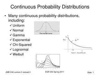
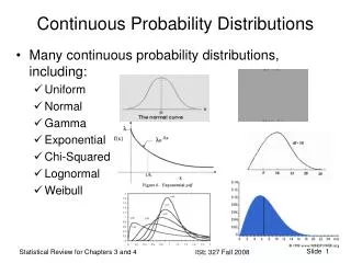
This document explores key aspects of continuous probability distributions, focusing on the Uniform and Normal distributions. It explains fundamental concepts such as probability density functions, expected values, variances, and the relationship between random variables. Practical examples illustrate the application of these distributions in real-world scenarios, including measurements in electrical engineering and quality control in manufacturing. The content also covers standard normal distribution, highlighting the significance of z-scores and their utility in probability calculations. ###

E N D
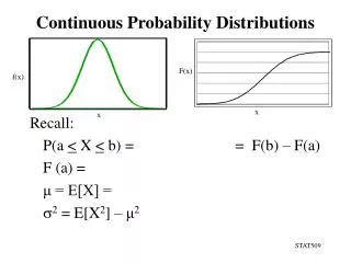
Continuous Probability Distributions Recall: P(a < X < b) = = F(b) – F(a) F (a) = μ = E[X] = s2 = E[X2] – μ2 F(x) f(x) x x STAT509
Continuous Uniform Distribution f(x;A,B) = 1/(B-A), A < x < B where [A,B] is an interval on the real number line μ = (A + B)/2 and s2 = (B-A)^2/12 1/(B-A) STAT509
Continuous Uniform Distribution • EX: Let X be the uniform continuous random variable that denotes the current measured in a copper wire in milliamperes. 0 < x < 50 mA. The probability density function of X is uniform. • f(x) = , 0 < x < 50 • What is the probability that a measurement of current is between 20 and 30 mA? • What is the expected current passing through the wire? • What is the variance of the current passing through the wire? STAT509
Normal Distribution n(x;μ,σ) = E[X] = μ and Var[X] = s2 f(x) x STAT509
Normal Distribution • Many phenomena in nature, industry and research follow this bell-shaped distribution. • Physical measurements • Rainfall studies • Measurement error • There are an infinite number of normal distributions, each with a specified μ and s. STAT509
Normal Distribution • Characteristics • Bell-shaped curve • - < x < + • μ determines distribution location and is the highest point on curve • Curve is symmetric about μ • s determines distribution spread • Curve has its points of inflection at μ +s • μ + 1s covers 68% of the distribution • μ + 2s covers 95% of the distribution • μ + 3s covers 99.7% of the distribution STAT509
Normal Distribution s s s s μ STAT509
Normal Distribution n(x; μ = 0, s = 1) n(x; μ = 5, s = 1) f(x) x STAT509
Normal Distribution n(x; μ = 0, s = 0.5) f(x) n(x; μ = 0, s = 1) x STAT509
Normal Distribution n(x; μ = 5, s = .5) f(x) n(x; μ = 0, s = 1) x STAT509
Normal Distribution μ + 1s covers 68% μ + 2s covers 95% μ + 3s covers 99.7% STAT509
Standard Normal Distribution The distribution of a normal random variable with mean 0 and variance 1 is called a standard normal distribution. STAT509
Standard Normal Distribution • The letter Z is traditionally used to represent a standard normal random variable. • z is used to represent a particular value of Z. • The standard normal distribution has been tabularized. STAT509
Standard Normal Distribution Given a standard normal distribution, find the area under the curve (a) to the left of z = -1.85 (b) to the left of z = 2.01 (c) to the right of z = –0.99 (d) to right of z = 1.50 (e) between z = -1.66 and z = 0.58 STAT509
Standard Normal Distribution Given a standard normal distribution, find the value of k such that (a) P(Z < k) = .1271 (b) P(Z < k) = .9495 (c) P(Z > k) = .8186 (d) P(Z > k) = .0073 (e) P( 0.90 < Z < k) = .1806 (f) P( k < Z < 1.02) = .1464 STAT509
Normal Distribution • Any normal random variable, X, can be converted to a standard normal random variable: z = (x – μx)/sx STAT509
Normal Distribution • Given a random Variable X having a normal distribution with μx = 10 and sx = 2, find the probability that X < 8. z x STAT509 4 6 8 10 12 14 16
Normal Distribution • EX: The engineer responsible for a line that produces ball bearings knows that the diameter of the ball bearings follows a normal distribution with a mean of 10 mm and a standard deviation of 0.5 mm. If an assembly using the ball bearings, requires ball bearings 10 + 1 mm, what percentage of the ball bearings can the engineer expect to be able to use? STAT509
Normal Distribution • EX: Same line of ball bearings. • What is the probability that a randomly chosen ball bearing will have a diameter less than 9.75 mm? • What percent of ball bearings can be expected to have a diameter greater than 9.75 mm? • What is the expected diameter for the ball bearings? STAT509
Normal Distribution • EX: If a certain light bulb has a life that is normally distributed with a mean of 1000 hours and a standard deviation of 50 hours, what lifetime should be placed in a guarantee so that we can expect only 5% of the light bulbs to be subject to claim? STAT509
Normal Distribution • EX: A filling machine produces “16oz” bottles of Pepsi whose fill are normally distributed with a standard deviation of 0.25 oz. At what nominal (mean) fill should the machine be set so that no more than 5% of the bottles produced have a fill less than 15.50 oz? STAT509
Relationship between the Normal and Binomial Distributions • The normal distribution is often a good approximation to a discrete distribution when the discrete distribution takes on a symmetric bell shape. • Some distributions converge to the normal as their parameters approach certain limits. • Theorem 6.2: If X is a binomial random variable with mean μ = np and variance s2 = npq, then the limiting form of the distribution of Z = (X – np)/(npq).5 as n , is the standard normal distribution, n(z;0,1). STAT509
Relationship between the Normal and Binomial Distributions • Consider b(x;15,0.4). Bars are calculated from binomial. Curve is normal approximation to binomial. STAT509
Relationship between the Normal and Binomial Distributions • Let X be a binomial random variable with n=15 and p=0.4. • P(X=5) = ? • Using normal approximation to binomial: n(3.5<x<4.5;μ=6, s=1.897) = ? Note, μ = np = (15)(0.4) = 6 s = (npq).5 = ((15)(0.4)(0.6)).5 = 1.897 STAT509
Relationship between the Normal and Binomial Distributions • EX: Suppose 45% of all drivers in a certain state regularly wear seat belts. A random sample of 100 drivers is selected. What is the probability that at least 65 of the drivers in the sample regularly wear a seatbelt? STAT509