Download
1 / 67
690 likes | 1.12k Views
Compiling for EDGE Architectures: The TRIPS Prototype Compiler. Kathryn McKinley Doug Burger, Steve Keckler, Jim Burrill 1 , Xia Chen, Katie Coons, Sundeep Kushwaha, Bert Maher, Nick Nethercote, Aaron Smith, Bill Yoder et al. The University of Texas at Austin

E N D
Compiling for EDGE Architectures:The TRIPS Prototype Compiler Kathryn McKinley Doug Burger, Steve Keckler, Jim Burrill1, Xia Chen, Katie Coons, Sundeep Kushwaha, Bert Maher, Nick Nethercote, Aaron Smith, Bill Yoder et al. The University of Texas at Austin 1University of Massachusetts, Amherst
Technology Scaling Hitting the Wall Qualitatively … Analytically … 35 nm 70 nm 100 nm 130 nm 20 mm chip edge Either way … Partitioning for on-chip communication is key
OO SuperScalars Out of Steam Clock ride is over • Wire and pipeline limits • Quadratic out-of-order issue logic • Power, a first order constraint Problems for any architectural solution • ILP - instruction level parallelism • Memory and on-chip latency Major vendors ending processor lines
OO SuperScalars Out of Steam Clock ride is over • Wire and pipeline limits • Quadratic out-of-order issue logic • Power, a first order constraint Problems for any architectural solution • ILP - instruction level parallelism • Memory and on-chip latency Major vendors ending processor lines What’s next?
Post-RISC Solutions • CMP - An evolutionary path • Replicate what we already have 2 to N times on a chip • Coarse grain parallelism • Exposes the resources to the programmer and compiler • Explicit Data Graph Execution (EDGE) 1. Program graph is broken into sequence of blocks • Blocks commit atomically or not - a block never partially commits 2. Dataflow within a block, ISA support for direct producer-consumer communication • No shared named registers (point-to-point dataflow edges only) • Memory is still a shared namespace • The block’s dataflow graph (DFG) is explicit in the architecture
Outline • TRIPS Execution Model & ISA • TRIPS Architectural Constraints • Compiler Structure • Spatial Path Scheduling
write read write read Gtile addi addi D[0] bro_t addi mov write addi lw_f mov addi bro_t lw_f Gtile D[0] addi write Block Atomic Execution Model TRIPS block Flow Graph Dataflow Graph Execution Substrate add add ld cmp read Register File write read read shl ld cmp br ld shl sw br Data Caches write read sw sw add br write • TRIPS block - single entry constrained hyperblock • Dataflow execution w/ target position encoding
TRIPS Block Constraints Fixed Size: 128 instructions • Padded with no-ops if needed Load/Store Identifiers: 32 load or store queue identifiers • More than 32 static loads and stores is possible Registers: 32 reads and 32 writes, 8 to each of 4 banks (in addition to 128) Register banks 32 reads 32 writes 32 loads 32 stores 1 - 128 instruction DFG Memory Memory PC read PC terminating branch PC • Constant Output: all stores and writes execute, one branch • Simplifies hardware logic for detecting block completion • Every path of execution through a block must produce the same stores and register writes Simplifies the hardware, more work for the compiler
Compiler Phases (Classic) TIL: TRIPS Intermediate Language - RISC-like three-address form TASL: TRIPS Assembly Language - dataflow target form w/ locations encoded PRE Global Value Numbering Scalar Replacement Global Variable Replacement SCC Copy Propagation Array Access Strength Reduction LICM Tree Height Reduction Useless Copy Removal Dead Variable Elimination Scale Compiler (UTexas/UMass) C FORTRAN Frontend Inlining Unrolling/Flattening Scalar Optimizations Code Generation Alpha TRIPS TIL SPARC PPC
Backend Compiler Flow Hyperblock Formation If-conversion Loop peeling While loop unrolling Instruction merging Predicate optimizations TIL Resource Allocation Register allocation Reverse if-conversion & split Load/Store ID assignment SSA for constant outputs Scheduling Fanout insertion Instruction placement Target form generation TASL
Correctness:Progressively Satisfy Constraints Constraint 128 instructions 32 load/store IDs 32 reg. read/write (8 per 4 banks) constant output Hyperblock Formation If-conversion Loop peeling While loop unrolling Instruction merging Predicate optimizations TIL Resource Allocation Register allocation Reverse if-conversion & split Load/Store ID assignment SSA for constant outputs Scheduling Fanout insertion Instruction placement Target form generation TASL
P Predication & Hyperblock Formation Predication • Convert control dependence to data dependence • Improves instruction fetch bandwidth • Eliminates branch mispredictions • Adds overhead • Any instruction can have a predicate, but... • Predicate head (low power) or bottom (speculative) Hyperblock • Scheduling region (set of basic blocks) • Single entry, multiple exit, predicated instructions • Expose parallelism w/o over saturating resources • Must satisfy block constraints head bottom P P
Accuracy? Constraint 128 instructions 32 load/store IDs 32 reg. read/write (8 per 4 banks) constant output Hyperblock Formation If-conversion Loop peeling While loop unrolling Instruction merging Predicate optimizations TIL Resource Allocation Register allocation Reverse if-conversion & split Load/Store ID assignment SSA for constant outputs Scheduling Fanout insertion Instruction placement Target form generation TASL
write read write read Gtile addi addi D[0] bro_t addi mov write addi lw_f mov addi bro_t lw_f Gtile D[0] addi write Block Atomic Execution Model TRIPS block Flow Graph Dataflow Graph Execution Substrate add add ld cmp read Register File write read read shl ld cmp br ld shl sw br Data Caches write read sw sw add br write TRIPS block - single entry constrained hyperblock Dataflow execution w/ target position encoding
add mul mul ld ld ld ld mul mul add st Spatial Scheduling Problem Partitioned microarchitecture
add ld mul mul ld ld ld ld ld mul mul st ld ld add st Spatial Scheduling Problem Partitioned microarchitecture Anchor points
add ld mul add mul mul mul ld mul ld ld ld ld mul mul st add ld ld add mul st Spatial Scheduling Problem Balance latency and concurrency Partitioned microarchitecture Anchor points
Outline • Background • Spatial Path Scheduling • Simulated Annealing • Extending SPS • Conclusions and Future Work
Static Dynamic VLIW (SPSI) Bad idea (DPSI) Static TRIPS (SPDI) Superscalars (DPDI) Dynamic Dissecting the Problem • Scheduling can have two components • Placement: Where an instruction executes • Issue: When an instruction executes Placement Issue EDGE
i3 i2 i1 i2 i2 i2 Explicit Data Graph Execution • Block-atomic execution • Instruction groups fetch, execute, and commit atomically • Direct instruction communication • Explicitly encode dataflow graph by specifying targets RISC EDGE R4 R5 R6 add r1, r4, r5 add r2, r5, r6 add r3, r1, r2 i1: addi3 i2: add i3 i3: add i4 add add Centralized Register File add
R0 R1 R2 R3 Ctrl E0 E1 E2 E3 D0 E4 E5 E6 E7 D1 E8 E9 E10 E11 D2 E12 E13 E14 E15 D3 Scheduling for TRIPS • TRIPS ISA • Up to 128 instructions/block • Any instruction can be in any slot • TRIPS microarchitecture • Up to 8 blocks in flight • 1 cycle latency between adjacent ALUs • Known • Execution latencies • Lower bound for communication latency • Unknown (estimated) • Memory access latencies • Resource conflicts Register File Data Cache
R0 R1 R2 R3 Ctrl D0 E2 D1 E4 D2 D3 Scheduling for TRIPS • TRIPS ISA • Up to 128 instructions/block • Any instruction can be in any slot • TRIPS microarchitecture • Up to 8 blocks in flight • 1 cycle latency between adjacent ALUs • Known • Execution latencies • Lower bound for communication latency • Unknown • Memory access latencies • Resource conflicts Register File Data Cache
Greedy Scheduling for TRIPS • GRST [PACT ‘04]: Based on VLIW list-scheduling • Augmented with five heuristics • Prioritizes critical path (C) • Reprioritizes after each placement (R) • Accounts for data cache locality (L) • Accounts for register output locality (O) • Load balancing for local issue contention (B) • Drawbacks • Unnecessary restrictions on scheduling order • Inelegant and overly specific Replace heuristics with elegant approach designed for spatial scheduling
Greedy Scheduling for TRIPS • GRST [PACT ‘04]: Based on VLIW list-scheduling • Augmented with five heuristics • Prioritizes critical path (C) • Reprioritizes after each placement (R) • Accounts for data cache locality (L) • Accounts for register output locality (O) • Load balancing for local issue contention (B) • Drawbacks • Unnecessary restrictions on scheduling order • Inelegant and overly specific Replace heuristics with elegant approach designed for spatial scheduling
Outline • Background • Spatial Path Scheduling • Simulated Annealing • Extending SPS • Conclusions and Future Work
read add mul ctrl R1 R2 br ld ld D0 ld add mul D1 ld mul add D0 D1 ctrl br read mul Legend add Register Data cache write Execution Control Spatial Path Scheduling Overview Scheduler Dataflow Graph Placement Topology
read add mul br ld ld D0 D1 ctrl read mul Legend add Register Data cache write Execution Control Spatial Path Scheduling Overview R1 add mul Scheduler Dataflow Graph ctrl D0 D1 R2 mul ld ld Placement Topology
read add mul br ld ld add R1 mul R2 add ld mul ld br D0 D1 ctrl D0 D1 read mul Legend add Register Data cache write Execution Control Spatial Path Scheduling Overview Scheduler Dataflow Graph Placement Topology
read R2 add mul br ld ld read R1 mul add write R1 Spatial Path Scheduling Overview Initialize all known anchor points Until all instructions are scheduled: • Populate the open list • Find placement costs • Choose the minimum cost location • Schedule the instruction whose minimum placement cost is largest (Choose the max of the mins)
read R2 add mul br ld ld ctrl R1 R2 D0 D1 ctrl D0 read R1 mul Legend D1 Register add Data cache Execution write R1 Control Unplaced Spatial Path Scheduling Example • Initialize all known anchor points Register File Data Cache
read R2 add mul br ld ld D0 D1 ctrl read R1 mul add write R1 Spatial Path Scheduling Example • Populate the open list (marked in yellow) Open list: Instructions that are candidates for scheduling We include: Instructions with no parents, or with at least one placed parent
read R2 1 add mul 3 br ld ld 1 D0 D1 ctrl 3 read R1 mul 3 add 1 write R1 1 Spatial Path Scheduling Example • Calculate placement cost for each instruction in the open list at each slot Placement cost(i,slot): Longest path length through i if placed at slot cost = inputCost + execCost + outputCost (includes communication and execution latencies)
read R2 1 mul 3 ld 1 D1 3 mul 3 add 1 write R1 1 Spatial Path Scheduling Example • Calculate placement cost for each instruction in the open list at each slot 5 Register File ctrl R1 R2 1 cycle D0 mul E1 3 3 cycles D1 5 cycles Data Cache 1 Total placement cost = 16 + 3 + 3 = 22
read R2 add mul br ld ld ctrl R1 R2 D0 D1 ctrl D0 22 22 24 26 read R1 mul D1 22 22 24 26 add 24 24 26 28 write R1 26 26 28 30 Spatial Path Scheduling Example • Calculate placement cost for each instruction in the open list at each slot Register File Data Cache
read R2 add mul br ld ld ctrl R1 R2 D0 D1 ctrl D0 22 22 24 26 read R1 mul D1 22 22 24 26 add 24 24 26 28 write R1 26 26 28 30 Spatial Path Scheduling Example • Choose the minimum cost location for each instruction Register File Data Cache
read R2 add mul br ld ld ctrl R1 R2 D0 D1 ctrl D0 22 22 24 26 read R1 mul D1 22 22 24 26 add 24 24 26 30 write R1 26 26 28 30 Spatial Path Scheduling Example • Break ties • Example heuristics: • Links consumed • ALU utilization Register File Data Cache
read R2 add mul br ld ld D0 D1 ctrl read R1 mul add write R1 Spatial Path Scheduling Example • Place the instruction with the highest minimum cost (Choose the max of the mins) Register File ctrl R1 R2 D0 mul D1 Data Cache
Spatial Path Scheduling Algorithm Schedule (block, topology) initialize known anchor points while (not all instructions scheduled) for each instruction in open list, i for each available location, n calculate placement cost for (i, n) keep track of n with min placement cost keep track of i with highest min placement cost schedule i with highest min placement cost Per-block complexity: SPS: O(i2 * n) i = # of instructions n = # of ALUs GRST: O(i2 + i * n) Exhaustive search: i !
SPS Benefits and Limitations • Benefits • Automatically exploits known communication latencies • Designed for spatial scheduling • Minimizes critical path length at each step • Naturally encompasses four of five GRST heuristics • Limitations of basic algorithm • Does not account for resource contention • Uses no global information • Minimum communication latencies may be optimistic
Experimental Methodology • 26 hand-optimized microbenchmarks • Extracted from SPEC2000, EEMBC, Livermore Loops, MediaBench, and C libraries • Average dynamic instructions fetched/block: 67.3 (Ranges from 14.5 to 117.5) • Cycle-accurate simulator • Within 4% of RTL on average • Models communication and contention delays • Comparison points • Greedy Scheduling for TRIPS (GRST) • Simulated annealing
SPS Performance Geometric mean of speedup over GRST: 1.19 Basic SPS
SPS Performance Geometric mean of speedup over GRST: 1.19 Basic SPS
SPS Performance Geometric mean of speedup over GRST: 1.19 Basic SPS
Outline • Background • Spatial Path Scheduling • Simulated Annealing • Extending SPS • Conclusions and Future Work
How well can we do? • Simulated annealing • Artificial intelligence search technique • Uses random perturbations to avoid local optima • Approximates a global optimum • Cost function: simulated cycles • Uncertainty makes static cost functions insufficient • Best cost function • Purpose • Optimization • Discover performance upper bound • Tool to improve scheduler
Speedup with Simulated Annealing Geometric mean of speedup over GRST Basic SPS: 1.19 Annealed: 1.40 Basic SPS Annealed
Speedup with Simulated Annealing Geometric mean of speedup over GRST Basic SPS: 1.19 Annealed: 1.40 Basic SPS Annealed
Speedup with Simulated Annealing Geometric mean of speedup over GRST Basic SPS: 1.19 Annealed: 1.40 Basic SPS Annealed
Outline • Background • Spatial Path Scheduling • Simulated Annealing • Extending SPS • Conclusions and Future Work
Extending SPS • Contention • Network link contention • Local and Global ALU contention • Global register prioritization • Path volume scheduling