Understanding Portfolio Allocation with Many Risky Assets and Efficient Diversification
This chapter explores the principles of efficient diversification in portfolio allocation involving multiple risky assets. It highlights the concept of the efficient frontier and the intuition behind constructing a tangency portfolio based on expected returns and standard deviations. By utilizing techniques such as the Sharpe ratio maximization and regression estimates, we can distinguish between systematic and unsystematic risks in portfolios. The chapter also illustrates how diversification cancels out fluctuations, ensuring better risk management and optimized returns in volatile markets.

Understanding Portfolio Allocation with Many Risky Assets and Efficient Diversification
E N D
Presentation Transcript
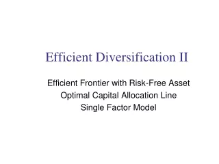
14-Efficient Diversification II BKM: Chapter 6
Portfolio Allocation • What about the case of many risky assets? • The efficient frontier has the same shape • Intuition is the same Tangency Portfolio Expected Return Individual Assets Best possible CAL risk free rate Standard Deviation
Multiple Assets Given time series of returns for n stock, you can find the portfolio with maximum Sharpe ratio as follows: • Pick arbitrary weights. • For the last stock, specify weight as 1-sum of others • Find the portfolio return using these arbitrary weights for each date (point to cells with weights) • Estimate the expected return and standard deviation • Calculate the Sharpe ratio of the portfolio • Use solver: maximize Sharpe ratio of portfolio by changing cells containing weights. Change all weights except last, which equals 1-sum of others
Diversification • In any portfolio, what fluctuations are “cancelled out”? • Simple two-stock example:
Portfolio Variance wMSFT ´ wDELL ´
Remaining Components wMSFT ´ wDELL ´
Portfolio Variance wMSFT ´ wDELL ´
Vanishing Components wMSFT ´ wDELL ´
Diversification • Portfolio Rule #5 • The component of the stock return that is independent of the portfolio return is always “off-set” or “canceled out” in a portfolio.
Diversification Vanishing Component Remaining Component Remaining Component Vanishing Component
Market Portfolio Assume the portfolio we hold is the market portfolio. When we combine stocks into this portfolio, again there is a “remaining” and “vanishing” component to each stock. We find this component for each stock by estimating the regression:
Market portfolio When we estimate this regression using a stock return as the “y” variable and the market return as the “x” variable, we call the slope coefficient beta (b) We call the variance of the remaining component “systematic risk” We call the variance of the vanishing component “unsystematic” or idiosyncratic, or “firm specific” risk.
Diversification and Many Risky Assets • R-square in this regression is • R-square in this regression is therefore the fraction of the total stock variance that “remains” or that is systematic.
Risk • Systematic risk refers to fluctuations in asset prices caused by macroeconomic factors that are common to all risky assets; hence systematic risk is often referred to as market risk. Examples of systematic risk factors include the business cycle, inflation, monetary policy and technological changes. • Firm-specific risk refers to fluctuations in asset prices caused by factors that are independent of the market, such as industry characteristics or firm characteristics. Examples of firm-specific risk factors include litigation, patents, management, and financial leverage.