Download
1 / 21
220 likes | 356 Views
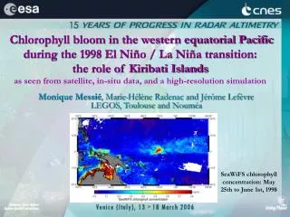
Chlorophyll bloom in the western equatorial Pacific during the 1998 El Niño / La Niña transition: the role of Kiribati Islands as seen from satellite, in-situ data, and a high-resolution simulation. Monique Messié , Marie-Hélène Radenac and Jérôme Lefèvre LEGOS, Toulouse and Nouméa.

E N D
Chlorophyll bloom in the western equatorial Pacific during the 1998 El Niño / La Niña transition: the role of Kiribati Islands as seen from satellite, in-situ data, and a high-resolution simulation Monique Messié, Marie-Hélène Radenac and Jérôme LefèvreLEGOS, Toulouse and Nouméa SeaWiFS chlorophyll concentration: May 25th to June 1st, 1998
Hypothesis from previous studies • Context at the beginning of 1998: - nitrate-limited ecosystem (Chavez et al., 1999), shallow nutricline - reappearance of the EUC (source of iron, Gordon et al., 1997 ) • Mechanisms: wind-driven upwelling and vertical mixing(Murtugudde et al., 1999; Wilson and Adamec, 2001; Ryan et al., 2002) • the bloom mechanisms appear to be quite well understood BUT • nutricline and EUC shoaling occurred in the whole equatorial Pacific • strongest easterlies near the dateline • why did the bloom occur in this particular region?
What we observe… SeaWiFS chlorophyll concentration (left), Topex-ERS SLA (top right), TMI SST (down rigth) : March 22th to 28th, 1998. White stars: TAO buoys.
Tarawa/Abaiang AbaiangTarawa Kiribati Islands as seen by MODIS(http://visibleearth.nasa.gov) Kiribati Islands SeaWiFS chlorophyll concentration: March 22th to 28th, 1998. White stars: TAO buoys.
Aim of the study to assess whether the islands played any role in the bloom generation and development Outline - Data and model presentation - Bloom chronology bloom generation bloom peak bloom demise - Conclusions • impact on the dynamics of the region • perturbations induced on nutrient fields and chlorophyll concentrations
Data • Satellite data: • surface chlorophyll concentration (SeaWiFS, 1/10°, 8-day) • SLA (Topex/Poseidon-ERS, 1/3°, weekly) • SST (TMI, 1/4°, weekly) SeaWiFS chlorophyll concentration: March 22th to 28th, 1998. White stars: TAO buoys. • In-situ data: TAO moorings at 165°E and 180° • temperature profiles • current profiles at 165°E, 0°
Run K: bathymetry Model • Regional Ocean Modeling System (ROMS): split-explicit, free-surface, σ-coordinate (Shchepetkin and McWilliams, 2005) • grid: 160°E-178°W, 6°S-11°N, 1/6°, 30 vertical levels2 grids (smoothed ETOPO2 bathymetry): - with islands: run Kiribati (K), land masking - with no islands: run No Kiribati (NK) • period:1996-1998 • boundary forcing: ORCA2 configuration of the OPA model • surface forcing: daily wind stress (TAO-ERS), 6-hour NCEP reanalysis • Regional Ocean Modeling System (ROMS): split-explicit, free-surface, σ-coordinate (Shchepetkin and McWilliams, 2005) • grid: 160°E-178°W, 6°S-11°N, 1/6°, 30 vertical levels2 grids (smoothed ETOPO2 bathymetry): - with islands: run Kiribati (K), land masking - with no islands: run No Kiribati (NK) • period:1996-1998 • boundary forcing: ORCA2 configuration of the OPA model • surface forcing: daily wind stress (TAO-ERS), 6-hour NCEP reanalysis
165°E-0°N: Uzonal (m s-1, color) and temperature (°C, black contours) Model validation Surface data: SST (TMI), SLA (Topex/Poseidon-ERS) TAO data: temperature and Uzonal profiles • Globally good agreement for surface and TAO data BUT: • EUC too weak, shoaling too late • cold bias in the bloom region
(data results) 1. Bloom generation:an island mass effect? • data results: island mass effect, impact on SLA • model results: islands impact on dynamics and nitrate-rich water masses islands position Bloom evolution 0°N-2°N averaged (December 1997 – September 1998) bloom demise bloom peak: a sudden input of iron? bloom generation:an island mass effect?
1. bloom generation 400 U incident current speed 0.5 m.s-1L dimension of the island 80 kmν horizontal eddy viscosity 100 m²s-1 Island mass effect (data results) • increase of chlorophyll concentration and biological productivity downstream of an oceanic island Study of the Tarawa/Abaiang island:low-latitude island characteristics of the wake predictable from Reynolds number (Heywood et al., 1996) • possible mechanism: flow disturbance eddies formation increased vertical mixing threshold for eddy sheding 70 a vortex street of eddies is supposed to occur downstream of the Tarawa/Abaiang group of islands
1. bloom generation Effect on SLA (data results) signature of eddies? vertical mixing and increased productivity Topex/Poseidon - ERS Sea Level Anomalies: January 5th to June 14th, 1998.
1. bloom generation °C °C Run K output: surface temperature (color) and currents (arrows), March 26th to 30th, 1998 Run K output: surface temperature (color) and currents (arrows), March 26th to 30th, 1998 24°C-isotherm depth averaged between 0°N and 2°N and EUC depth (March-April 1998) Islands impact on dynamics (model results) In the wake of the islands: • cold SST, low SSH and high water density • meanders and eddies • shoaling of temperature isolines in the upper part of the thermocline; same for density isolines and EUC
1. bloom generation SeaWiFS data Run K PasTr 0°N-2°N PasTr average (dimensionless). White contour : bloom area (0.3 and 0.5 mg m-3 iso-[Chl]) SeaWiFS Chl concentration (mg m-3): March 22th to 28th, 1998. Run K, N-tracer: March 24th to 28th, 1998. Nitrate-type passive tracer (model results) Passive tracer: [PasTr] = 0 for T > 24°C[PasTr] = 27 – 1.1235 T for T 24°C
1. bloom generation local changesvertical advection horizontal advection vertical mixing 0°N-2°N passive tracer diagnostics(50 m upper layer): bloom generation (24/02-20/04) longitude Processes at work (model results) near the islands position: vertical advection at the bloom location: vertical advection and vertical mixing
(data results) 2. Bloom peak:a sudden input of iron? • data results: TAO data at 165°E, 0°N • model results: islands impact on the EUC and iron-type lagrangian floats islands position Bloom evolution 0°N-2°N averaged (December 1997 – September 1998) bloom demise bloom peak: a sudden input of iron? bloom generation:an island mass effect?
2. bloom peak bloom peak TAO data 165°E-0°N: Uzonal (m s-1, color) and temperature (°C, black contours) TAO data (data results) • end of April: current reversal at 40m depth weakening of the island mass effect cannot explain the highest Chl concentrations • current reversal: because of the potential iron-rich EUC shoaling sudden input of iron?
2. bloom peak 0 Run K Run NK temporal distribution Example of Fe-floats initial position (March 28th, 160°E). Black lines: zonal current isolines. depth (m) Run K Run NK spatialdistribution -500 -5 0 5 latitude Iron-type lagrangian floats (model results) injection in the EUC at the western boundary, for z < -80 m and u > 80% max(uEUC), every 10 days from January 27th to June 6th. results: study of the first appearance of Fe-floats in the 50 m upper layer
(data results) 3. Bloom demise:eastward advection of chlorophyll-poor waters? • data and model surface current • passive tracer diagnostics islands position Bloom evolution 0°N-2°N averaged (December 1997 – September 1998) bloom demise bloom peak: a sudden input of iron? bloom generation:an island mass effect?
3. bloom demise (model results) bloom demise local changesvertical advection horizontal advection vertical mixing 0°N-2°N passive tracer diagnostics in June (50 m upper layer) longitude Horizontal advection (data results) TAO data 165°E-0°N: Uzonal (m s-1, color) and temperature (°C, black contours) probably surface current reversal in June eastward current during the bloom demise horizontal advection drives the bloom demise
Conclusion:bloom sequence mg m-3 demise bloom generation (Jan-Apr):island mass effect eddies, vertical mixing + wind-driven upwelling nitrate input peak generation bloom peak (Apr-May):EUC shoaling enhanced by the presence of the islands barrier sudden input of iron dramatic increase of chlorophyll concentration bloom demise (May-Jun):EUC surfacing surface currents reversal eastward advection of nutrient-poor waters
Conclusion • Influence of Kiribati Islands on the bloom generation and development: - disruption of the dynamics and nutrient fields - responsible for the strength and location of nitrate and iron inputs • Need of a coupled physical/biological model