Download
1 / 42
420 likes | 441 Views
Learn about the Normal and Standardized Normal distributions, the Binomial Approximation, sample data, populations vs. samples, and sample measures in statistics.

E N D
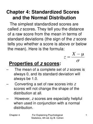
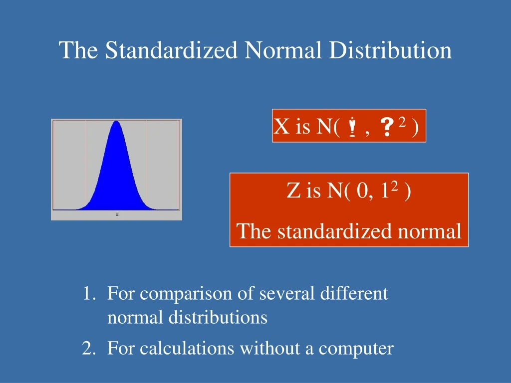
The Standardized Normal Distribution X is N( , 2 ) Z is N( 0, 12 ) The standardized normal • For comparison of several different normal distributions • For calculations without a computer
The Normal Approximationto the Binomial Both distributions have the same shape…
This normal approximation to the binomial works reasonably well when • np 5 and n(1-p) 5 • No computer is nearby But it is important fact that the binomial distribution and normal distribution are similar … we will return to this subject relatively soon … central limit …
Conceptual idea of new topics When talking about binomial and normal probabilities, we’ve taken the following point of view: A situation follows certain “probabilities,” and we can use this knowledge to deduce specific information about the situation Now we will take the reverse point of view: Specific information about a situation can be used to find “probabilities” that describe the situation The word “features” could replace “probabilities”
For example, think about the quiz you took… Professors have always noticed that students’ scores on a test tend to follow a normal distribution By actually giving a test to a sample of students, you can estimate the mean and standard deviation of the underlying normal distribution For tests like the SAT, the underlying distribution is then used as a ranking measure for students taking the same test later These ideas are loose, and first we’re going to learn how to work with sample data
Populations and Samples A population is a complete set of data representing a given situation A sample is a subset of the population --- ideally a small-scale replica of the population E.g., all students that take the SAT constitute a population, while those taking the test on a particular Saturday are a sample E.g., all American citizens are a population, while those selected for a survey are a sample Populations are a relative concept
For the following definitions, imagine a population like the starting salaries of all MBA students graduating this year A population is assumed to follow a random variable X, with values and probabilities X = starting salary of a particular MBA student P(X = $100,000) = ???? So we could calculate the expected value of the population, as well as the standard deviation Except it is sometimes hard to get a handle on the entire population. Imagine finding out the starting salaries of every single graduating MBA student in the U.S.!
So instead of trying to look at the entire population, we look at a sample of the population, which hopefully gives us a good picture of the population We might take a survey of graduating MBAs to determine the average (or expected) starting salary • A sample statistic is a quantitative measure of a sample; used to make estimates of the population • A sample mean (or expected value) is used to estimate the population mean • A sample standard deviation is used to estimate the population mean
sample mean = X = (X1 + X2 + … + Xn) / n Sample std dev = SX = sqrt ( [ (X1 – X)2 + (X2 – X)2 + … + (Xn – X)2 ] / (n-1) ) Summary/Sample Measures A sample is made up of n observations X1, X2, …, Xn The median is the middle of the values; 50% of the observation values fall below the median and 50% above The mode is the most frequent observation value The maximum and minimum are the largest and smallest observations; the range is the difference between the max and min
Relevant Excel Commands = AVERAGE(array) = STDEV(array) Tools Data Analysis Descriptive Statistics (see Excel file)
Setup and Assumptions for This Lecture • You have a population about which you’d like to know things such as mean, std dev, proportions • Each member of the population is assumed to follow the random variable X with mean X, std dev X, and particular proportion pX • Again, however, X, X, and pX are unknown • The population is too big to measure directly • You will take samples instead • What information can be deduced?
A Practical Approach: Point Estimates Here’s an idea… To estimate X, X, and pX, take a sample of size n and calculate sample mean X-bar, sample std dev SX, and sample proportion X/n. Use these as “point estimates” of the true X, X, and pX (a) Xi = value of i-th observation (b) Xi = 1 if i-th observations has attribute, 0 otherwise
Can we do better? Point estimates are nice, but is there a better idea? After all, who knows how close X-bar, SX, and X/n are to X, X, and pX? …interval estimates… For example, point estimate: “An estimate for the true mean X is the point estimate X-bar = 23.66.” For example, interval estimate: “There is a 95% probability that the true mean X lies between 23.60 and 23.70.” Interval estimates are stronger than point estimates
Yes, we can do better! But it takes the investigation of some pretty tricky concepts… the sampling random variable and the sampling distribution
The Sampling Random Variable and the Sampling Distribution Fix in your mind a number n – the number of observations taken in a single sample Now think about taking many different samples of size n and calculating the sample mean for each sample taken The sampling random variable is the random variable that assigns the sample mean to each sample of size n … And the sampling distribution is the distribution of this random variable
Key Facts about the Sampling Distribution The mean of the sampling distribution is the mean of the population The std dev of the sampling distribution is the std dev of the population divided by the square root of n If n is large then the sampling random variable is approximately normally distributed Central Limit Theorem
Comments on the Sampling Distribution Remember: we don’t actually know X or X and so we don’t know the mean and standard deviation of the sampling distribution either We can make statements like: “The sample mean of a random sample of size n has a 95% chance of falling within 2 std devs up or down from the true population mean” The standard deviation of the sampling distribution is commonly called the standard error
An Example We can make statements like: “The sample mean of a random sample of size n has a 95% chance of falling within 2 standard errors up or down from the true population mean” (see Excel) Again, we must stress that we don’t know true population mean, population std dev, or sampling distribution std error
How the Sampling Distribution Can Be Used If we don’t know anything about the sampling distribution except “in theory,” then how can we really use it? Well, we can determine some information about the sampling distribution by taking an actual sample of size n SX-bar is called the sample standard error
A Practical Approach: Interval Estimates (Means) Using a sample of size n, let X-bar serve as a point estimate of the true population mean X and of the mean X-bar of the sampling distribution Also let the sample standard error SX-bar serve as an estimate of the standard error of X-bar From this information, we can build “confidence intervals” for the true mean Xof the population
Confidence Intervals (Means) Using a single sample of size n 30 with information a 95% confidence interval for the actual population mean X is “We are 95% confident that the true population mean Xis between these two numbers.”
Confidence Intervals (Means) (cont’d) For a k% confidence interval, 1.960 is replaced with the value z having P(-z Z z) = 0.01*(100 - k): By formula, z = NORMSINV( 0.01*( 50 + k/2 ) ) Z is the standardized normal
Sample Problem The corresponding Excel file contains a sample of size 80 on the length of a precision shaft for use in lathes. • Calculate the mean, standard deviation, and standard error of the 80 values • Construct 95% and 99% confidence intervals (C.I.s) for the population mean (see Excel)
Confidence Intervals (Proportions) If you have then a 95% confidence interval for the true population proportion is The 1.960 follows the same rules as for means with n 30
The estimate is, therefore, a binomial random variable with : Mean = np/n = p And Standard Deviation = sqrt(np[1-p])/n = sqrt(p[1-p]/n) Note: We can apply the CLT to approximate the binomial with a normal having the same mean and standard deviation.
Central Limit Theorem Restated for Population Proportions • As the Sample size, n, increases, the sampling distribution approaches a normal distribution with • Mean = p • Standard deviation = sqrt[p (1 – p)/n]
Heart Valve Example Re-Visited • 79 out of 100 assemblies were good • Estimates for mean and stdev are: • Mean = 0.79 • Stdev = sqrt[0.79 (1 – 0.79)/100] = 0.040731
Example Problem Continued • Estimate the population proportion of lathes that exceed 6.625 inches. Construct a 90% C.I. for this proportion (see Excel)
Sample Size Needed to Achieve High Confidence (Means) Considering estimating X, how many observations n are needed to obtain a 95% confidence interval for a particular error tolerance? The error tolerance E is ½ the width of the confidence interval Here, is a conservative (high) estimate of the true std dev X, often gotten by doing a preliminary small sample 1.960 can be adjusted to get different confidences
Example Problem Continued • Consider the sample of 80 as a preliminary sample. Find the minimal sample size to yield a 95% C.I. for the population mean with E = 0.00005. What about for 99% confidence? (see Excel)
Sample Size Needed to Achieve High Confidence (Proportions) Considering estimating pX, how many observations n are needed to obtain a 95% confidence interval for a particular error tolerance? The error tolerance E is ½ the width of the confidence interval Here, p is a conservative (closer to 0.5) estimate of the true population proportion pX, often gotten by doing a preliminary small sample 1.960 can be adjusted to get different confidences
Polling Example In estimating the proportion of the population that approves of Bush’s performance as President, how many people should be polled to provide a 95% confidence interval with error 0.02? “83% of Americans approve of the job Bush is doing, plus or minus 2 percentage points” We should use conservative estimate of true proportion n = (1.960/0.02)^2 (0.5)(1 – 0.5) = 2401.0 But, if we’re certain px 0.6… n = (1.960/0.02)^2 (0.6)(1 – 0.6) = 1920.8