Download
1 / 34
400 likes | 719 Views
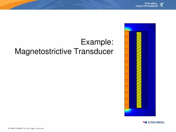
Example: Magnetostrictive Transducer. Introduction. This is a 2D axi-symmetric model of a magnetostrictive transducer. Magnetostrictive transduction is used in sonars, acoustic devices, active vibration and position control and fuel injection systems.

E N D
Introduction • This is a 2D axi-symmetric model of a magnetostrictive transducer. • Magnetostrictive transduction is used in sonars, acoustic devices, active vibration and position control and fuel injection systems. • The transducer has a steel housing enclosing a drive coil. A magnetostrictive material is placed in the core which works as an actuator when a magnetic field is produced by passing a current through the drive coil.
Magnetostrictive Transducer Sectional view of a cylindrical transducer Steel housing (for magnetic flux path) Drive coil (homogenous current carrying element) Magnetostrictive rod (active material)
Model Features • 2D axial symmetry used to reduce computation time. • Non-linear constitutive relation between magnetostriction and magnetic field is implemented. The material is assumed to be in a pre-stressed state that would yield maximum magnetostriction. • Non-linear B-H curve is used to model realistic magnetic behavior including saturation effect at high magnetic fields. • The drive coil is modeled as a homogenized current carrying domain. Individual wires are not resolved. • Magnetostatic modeling is performed. A parametric sweep of current density in the drive coil is used to demonstrate the non-linear magnetostriction vs. magnetic field.
Magnetostriction - Theory • Magnetostrictive materials exhibit free strain (λ) when exposed to magnetic field (H). This phenomena is known as the Joule effect. • This phenomena has a quantum mechanical origin. The magneto-mechanical coupling takes place at the atomic level. • From a system level, the material can be assumed to comprise of a number of tiny ellipsoidal magnets which rotate due to the torque produced by the externally applied magnetic field. • The rotation of these elemental magnets produce dimensional change as shown in this animation. Source: http://en.wikipedia.org/wiki/File:Magnetostriction_by_Zureks.gif
Magnetostriction – Effect of magnetic field • The free strain is often modeled using linear constitutive relation: λ = dH where d is called the piezo-magnetic strain coefficient. • In reality, the free strain (magnetostriction) has a non-linear dependence on the applied magnetic field and the mechanical stress in the material. Pre-stress Magnetostriction vs. Magnetic field at various pre-stresses Source: http://www.etrema-usa.com/documents/Terfenol.pdf
Physics 1 – Electromagnetic • AC/DC Module > Statics, Magnetic > Azimuthal Induction Currents, Vector Potential • Calculates the azimuthal magnetic potential (Aφ) for a given azimuthal current density (Jφ). • The magnetic problem is solved to find the spatial distribution of magnetization (Mr_emqa, Mz_emqa).
Physics 2 – Structural • Structural Mechanics Module > Axial Symmetry, Stress-Strain > Static analysis • Magnetostriction (Lambda_r, Lambda_z) values are assigned as initial strains (εri, εzi) in the magnetostrictive rod. • This creates a one-way coupling of the structural problem with the magnetic problem.
Geometry Steel housing Drive coil Magnetostrictive rod Air domain (required to view realistic magnetic flux path)
Dimensions Air (Subdomains 1, 4, 6) • Magnetostrictive rod • Radius = 3 mm • Height = 50 mm • Coil • Radius = 3 mm • Height = 50 mm • Steel housing • Head and base plates • Radius = 20 mm • Height = 5 mm • Side wall • Thickness = 5 mm • Height = 50 mm • Air domain • Radius = 90 mm • Height = 180 mm Steel housing (Subdomain 2) Current-carrying coil (Subdomain 5) Magnetostrictive rod (Subdomain 3)
Calculation of magnetostriction Ref: S. Chikazumi, “Physics of Ferromagnetism,” 2nd ed., Clarendon Press. • Magnetostriction (λi) along direction i depends on the magnetostriction constant (λs) and the magnetization direction cosine (αi). • The direction cosine is the ratio of magnetization along the required direction (Mi) and the saturation magnetization (Ms) of the material. • The negative 1/3 term indicates that the magnetic moments are randomly oriented in the material in the absence of any magnetic field. • We will not use this 1/3 term because we have assumed that the material is sufficiently pre-stressed such that all magnetic moments are perpendicular to the direction of magnetization at the beginning of the magnetization process.
Options > Expressions > Subdomain Expressions Note: Constitutive relation is applied only to subdomain 3 which represents the magnetostrictive material.
Subdomain settings - Magnetic • Make sure the application mode emqa is selected from the Multiphysics menu. • Subdomains 1, 4, 6 – No changes are necessary. • Subdomain 2 - Choose Library Material as “Soft iron (with losses).” Choose constitutive relation (H↔B) as H = f(|B|)eB. • Go to Options > Materials/Coefficients library. Expand Model(1) and click on Soft Iron (with losses)(mat1). In the sigma edit field, type 0.Click Apply and OK.
Subdomain settings - Magnetic • Subdomain 3 – Assume a non-linear but isotropic magnetostrictive material. Choose constitutive relation (H↔B) as H = f(|B|)eB. Type HBFe(normB_emqa[1/T])[A/m] in the H edit field. • HBFe is a user-defined function to model the non-linear B-H curve in the magnetostrictive material. • The B-H curve function can be created by the user using experimental material data. User-defined functions are created from Options > Functions.
Non-linear B-H Curve H = HBFe(B) H Interpolation table B
Subdomain settings - Magnetic • Subdomain 5 - Type J0 in the Jφe edit field. • Note that the electrical conductivity in subdomain 5 is set to zero because in reality the turns of wires in a drive coil are insulated from each other so that the current only flows along the circumferential direction (φ) and not along the axial (z) and radial (r) directions.
Boundary settings - Magnetic Magnetic Insulation (Boundaries 2, 11, 26) Axial Symmetry (Boundaries 1, 3, 5, 7, 9) This boundary condition sets the magnetic vector potential Aφ = zero. This is an approximation for a boundary at infinity. The user may also use infinite elements for a more high fidelity model. See the AC/DC Module User's Guide for information on infinite elements. All other boundaries - Continuity
Subdomain settings - Structural • Select the application mode smaxi from the Multiphysics menu • Deactivate all other Subdomains except Subdomain 3 by clearing the checkmark from the Active in this domain option. • Subdomain 3 – In the Material tab, type 60e9 [Pa] and 0.45 in the Young’s modulus and Poisson’s ratio edit fields respectively to simulate the mechanical properties of typical magnetostrictive material.
Subdomain settings - Structural • Subdomain 3 – Add the magnetostriction (Lambda_r and Lambda_z) using the Initial Stress and Strain tab.
Why initial strain? [σ] – Stress [C] – Stiffness [ε] – Strain [εi] - Initial strain [σi] - Initial stress Generalized Hooke’s Law • Magnetostriction does not produce stress in the material unless it is constrained. • Modeling magnetostriction as an initial strain ensures that the material remains stress-free when the strain in the body is the same as the magnetostriction.
Boundary settings - Structural Free – Boundaries 8 and 12 Axial symmetry – Boundary 5 Magnetostrictive rod (Subdomain 3) Fixed – Boundary 6
Meshing • It is desired to calculate the magnetic quantities in the magnetostrictive rod and steel housing with high accuracy. • Go to the Subdomain tab under Mesh > Free Mesh Parameters. Type 1e-3 in the Maximum element size edit field for subdomains 2 and 3. • Go to the Boundary tab under Free Mesh Parameters. Type 1e-4 in the Maximum element size edit field for boundaries 6 and 8. • Click the Remesh button followed by OK button.
Results Magnetic flux concentration through the magnetostrictive rod and steel housing depicted by the streamlines. • Uniform magnetic flux density inside the magnetostrictive rod along the centerline (r = 0). • Flux density tapers off sharply through the steel head and base plates.
Results Uniform axial strain (~ 1.47e-4) in the magnetostrictive rod due to magnetostriction. Zero axial stress in the magnetostrictive rod due to “free strain.” Uniform axial strain in the magnetostrictive rod along the centerline (r = 0)
Creating the non-linear λ vs. H curve • It is desired to find out the free strain of the magnetostrictive material or displacement obtained from the transducer as a function of the input current or input magnetic field for most applications. • To find this out we need to perform a parametric analysis. • Assume J0 varies “quasi-statically” so that there is no inductive effect and no skin-effect.
Solve > Solver Parameters • Use the settings shown here and click OK. • Click the = button to solve. • It will probably take a few minutes.
Plotting the non-linear λ vs. H curve • Postprocessing > Plot Parameters > Domain Plot Parameters. • In the General tab, make sure all the solutions are selected in the Solutions to use area. • Select the Point tab and choose point 4. • In the y-axis data area, type Lambda_z in the Expression edit field. • In the x-axis data area, select the Expression radio button and then click on the Expression button. Type Hz_emqa. Non-linear magnetostriction vs. magnetic field curve along the axial direction.
Plotting the displacement vs. input current density • Postprocessing > Plot Parameters > Domain Plot Parameters. • In the General tab, make sure all the solutions are selected in the Solutions to use area. • Select the Point tab and choose point 4. • In the y-axis data area, type w in the Expression edit field. • In the x-axis data area, select the Expression radio button and then click on the Expression button. Type J0. Non-linear axial displacement vs. input current density.
References • C. Mudivarthi, S. Datta, J. Atulasimha and A. B. Flatau, “A bidirectionally coupled magnetoelastic model and its validation using a Galfenol unimorph sensor,” Smart Materials and Structures, 17 035005 (8pp), 2008.http://www.iop.org/EJ/abstract/0964-1726/17/3/035005/ • F. Graham, “Development and Validation of a Bidirectionally Coupled Magnetoelastic FEM Model for Current Driven Magnetostrictive Devices,” M.S. Thesis, Aerospace Engineering, University of Maryland, College Park, USA, 2009.http://www.lib.umd.edu/drum/handle/1903/9354