Download
1 / 43
430 likes | 543 Views
CZ5225: Modeling and Simulation in Biology Lecture 6, Microarray Cancer Classification Prof. Chen Yu Zong Tel: 6874-6877 Email: csccyz@nus.edu.sg http://xin.cz3.nus.edu.sg Room 07-24, level 7, SOC1, National University of Singapore. Why Microarray?.

E N D
CZ5225: Modeling and Simulation in BiologyLecture 6, Microarray Cancer Classification Prof. Chen Yu ZongTel: 6874-6877Email: csccyz@nus.edu.sghttp://xin.cz3.nus.edu.sgRoom 07-24, level 7, SOC1, National University of Singapore
Why Microarray? • Although there has been some improvements over the past 30 years still there exists no general way for: • Identifying new cancer classes • Assigning tumors to known classes • In this paper they are introducing two general ways for • Class prediction of a new tumor • Class discovery of new unknown subclasses • Without using the previous biological information
Why Microarray? • Why do we need to classify cancers? • The general way of treating cancer is to: • Categorize the cancers in different classes • Use specific treatment for each of the classes • Traditional way • Morphological appearance.
Why Microarray? • Why traditional ways are not enough ? • There exists some tumors in the same class with completely different clinical courses • May be more accurate classification is needed • Assigning new tumors to known cancer classes is not easy • e.g. assigning an acute leukemia tumor to one of the • AML • ALL
Cancer Classification • Class discovery • Identifying new cancer classes • Class Prediction • Assigning tumors to known classes
Cancer Genes and Pathways • 15 cancer-related pathways, 291 cancer genes, 34 angiogenesis genes, 12 tumor immune tolerance genes Nature Medicine 10, 789-799 (2004); Nature Reviews Cancer 4, 177-183 (2004), 6, 613-625 (2006); Critical Reviews in Oncology/Hematology 59, 40-50 (2006) http://bidd.nus.edu.sg/group/trmp/trmp.asp
Most discriminative genes Patient i: Disease outcome prediction with microarray Patient SVM Important genes Normal person j: Normal Patient i: Signatures Predictor-genes Patient SVM Normal person j: Better predictive power Clues to disease genes, drug targets Normal
Patient i: Patient SVM Normal person j: Normal • Expected features of signatures: • Composition: • Certain percentages of cancer genes, genes in cancer pathways, and angiogenesis genes • Stability: • Similar set of predictor-genes in different patient compositions measures under the same or similar conditions Disease outcome prediction with microarray How many genes should be in a signature?
Class Prediction • How could one use an initial collection of samples belonging to known classes to create a class Predictor? • Gathering samples • Hybridizing RNA’s to the microarray • Obtaining quantitative expression level of each gene • Identification of Informative Genes via Neighborhood Analysis • Weighted votes
Neighborhood Analysis • We want to identify the genes whose expression pattern were strongly correlated with the class distinction to be predicted and ignoring other genes • Each gene is presented by an expression vector consisting of its expression level in each sample. • Counting no. of genes having various levels of correlation with ideal gene c. • Comparing with the correlation of randomly permuted c with it • The results show an unusually high density of correlated genes!
Idealized expression pattern Neighborhood analysis
Class Predictor • The General approach • Choosing a set of informative genes based on their correlation with the class distinction • Each informative gene casts a weighted vote for one of the classes • Summing up the votes to determine the winning class and the prediction strength
Computing Votes • Each gene Gi votes for AML or ALL depending on : • If the expression level of the gene in the new tumor is nearer to the mean of Gi in AML or ALL • The value of the vote is : • WiVi where: • Wi reflects how well Gi is correlated with the class distinction • Vi = | xi – (AML mean + ALL mean) / 2 | • The prediction strength reflects: • Margin of victory • (Vwin – Vloose) / (Vwin + Vloose)
Evaluation • DATA • Initial Sample • 38 Bone Marrow Samples (27 ALL, 11 AML) obtained at the time of diagnosis. • Independent Sample • 34 leukemia consisted of 24 bone marrow and 10 peripheral blood samples (20 ALL and 14 AML). • Validation of Gene Voting • Initial Samples • 36 of the 38 samples as either AML or ALL and two as uncertain. All 36 samples agrees with clinical diagnosis. • Independent Samples • 29 of 34 samples are strongly predicted with 100% accuracy.
An early kind of analysis: unsupervised learning learning disease sub-types p53 Rb
Sub-type learning: seeking ‘natural’ groupings & hoping that they will be useful… p53 Rb
E.g., for treatment Respond to treatment Tx1 p53 Do not Respond to treatment Tx1 Rb
The ‘one-solution fits all’ trap Do not Respond to treatment Tx2 p53 Rb Respond to treatment Tx2
Predictive Biomarkers & Supervised Learning Predictive Biomarkers
A more modern view 2: Unsupervised learning as structure learning
Causative biomarkers & (structural) unsupervised learning Causative Biomarkers
If 2D looks good, what happens in 3D? • 10,000-50,000 (regular gene expression microarrays, aCGH, and early SNP arrays) • 500,000 (tiled microarrays, SNP arrays) • 10,000-300,000 (regular MS proteomics) • >10, 000, 000 (LC-MS proteomics) This is the ‘curse of dimensionality problem’
Problems associated with high-dimensionality (especially with small samples) • Some methods do not run at all (classical regression) • Some methods give bad results • Very slow analysis • Very expensive/cumbersome clinical application
P O A E C D B K T H I J Q L M N Solution 2: feature selection
Another (very real and unpleasant) problem Over-fitting • Over-fitting ( a model to your data)= building a model than is good in original data but fails to generalize well to fresh data
Over-fitting is directly related to the complexity of decision surface (relative to the complexity of modeling task)
Over-fitting is also caused by multiple validations & small samples
Over-fitting is also caused by multiple validations & small samples
A method to produce realistic performance estimates: nested n-fold cross-validation
Datasets • Bhattacharjee2 - Lung cancer vs normals [GE/DX] • Bhattacharjee2_I - Lung cancer vs normals on common genes between Bhattacharjee2 and Beer [GE/DX] • Bhattacharjee3 - Adenocarcinoma vs Squamous [GE/DX] • Bhattacharjee3_I - Adenocarcinoma vs Squamous on common genes between Bhattacharjee3 and Su [GE/DX] • Savage - Mediastinal large B-cell lymphoma vs diffuse large B-cell lymphoma [GE/DX] • Rosenwald4 - 3-year lymphoma survival [GE/CO] • Rosenwald5 - 5-year lymphoma survival [GE/CO] • Rosenwald6 - 7-year lymphoma survival [GE/CO] • Adam - Prostate cancer vs benign prostate hyperplasia and normals [MS/DX] • Yeoh - Classification between 6 types of leukemia [GE/DX-MC] • Conrads - Ovarian cancer vs normals [MS/DX] • Beer_I - Lung cancer vs normals (common genes with Bhattacharjee2) [GE/DX] • Su_I - Adenocarcinoma vs squamous (common genes with Bhattacharjee3) [GE/DX • Banez - Prostate cancer vs normals [MS/DX]
Methods: Gene Selection Algorithms • ALL - No feature selection • LARS - LARS • HITON_PC - • HITON_PC_W -HITON_PC+ wrapping phase • HITON_MB - • HITON_MB_W -HITON_MB + wrapping phase • GA_KNN - GA/KNN • RFE - RFE with validation of feature subset with optimized polynomial kernel • RFE_Guyon - RFE with validation of feature subset with linear kernel (as in Guyon) • RFE_POLY - RFE (with polynomial kernel) with validation of feature subset with polynomial optimized kernel • RFE_POLY_Guyon - RFE (with polynomial kernel) with validation of feature subset with linear kernel (as in Guyon) • SIMCA - SIMCA (Soft Independent Modeling of Class Analogy): PCA based method • SIMCA_SVM - SIMCA (Soft Independent Modeling of Class Analogy): PCA based method with validation of feature subset by SVM • WFCCM_CCR - Weighted Flexible Compound Covariate Method (WFCCM) applied as in Clinical Cancer Research paper by Yamagata (analysis of microarray data) • WFCCM_Lancet - Weighted Flexible Compound Covariate Method (WFCCM) applied as in Lancet paper by Yanagisawa (analysis of mass-spectrometry data) • UAF_KW - Univariate with Kruskal-Walis statistic • UAF_BW - Univariate with ratio of genes between groups to within group sum of squares • UAF_S2N - Univariate with signal-to-noise statistic
Classification Performance (average over all tasks/datasets)
How well dimensionality reduction and feature selection work in practice?
Number of Selected Features (average over all tasks/datasets)
Number of Selected Features (average over all tasks/datasets)