Exact Methods for Allocating Operations with the Pinto Heuristic and B&B Algorithm
The ALB problem can be approached as a shortest path problem without developing a complete graph, utilizing operations assignment and dominance pruning. The Pinto heuristic considers subgraphs to offer feasible operation orderings based on precedence rules. Various priority rules aid in determining efficient orderings of operations. The Breadth-First (DP) and Depth-First (B&B) algorithms enable effective problem-solving through systematic exploration of operation assignments, ensuring optimal solutions like those found in the FABLE method for balancing lines.

Exact Methods for Allocating Operations with the Pinto Heuristic and B&B Algorithm
E N D
Presentation Transcript
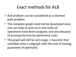
Exact methods for ALB • ALB problem can be considered as a shortest path problem • The complete graph need not be developed since one can stop as soon as in one node all operations have been assigned, and also because of pruning the tree by dominance rules • The graph will still bevery large -> heuristicthatconsidersonly a subgraphwiththecostofloosingguaranteeofoptimality
Pinto heuristic • Find some good (and feasible w.r.t. precedence) orderings of the operations using e.g. different priority rules • For each of these orderings (permutations) (jl,. ... , jn) of operations, define nodes (states) Z0 = {}, {jl}, {jl, j2}, ... , Zend = {jl, ... , jn}. • Draw an arrow from node Z to Z' if Z' - Z represents a feasible assignment of a station in the sense that cycle time is not exceeded: • In the resulting graph find the shortest path from Z0 = {} to Zend = {jl, ... , jn}.
Pinto heuristic • Example: c=4 Ordering 1: 2, 1, 4, 5, 3 Ordering 2: 1, 4, 5 ,2, 3 Bycoincidencethe optimal solutionisreached!
B&B algorithm by Johnson (FABLE) • DP algorithmcanbeconsideredas „breadth“ search • All nodes in a certainstageareconsidered, beforeproceedingtothenextstage • The firstcompletesolutionisalreadythe optimal one; ifthealgorithmisstoppedbecauseof time restrictionsnofeasiblesolutionisavailable. • -> B&B algorithmby Johnson treistosearchthecorrespondingtree in the sense of „depth“ searchbytryingtoreachleavesofthetreesoon (completesolution). • Algorithmis also knownas FABLE: fast algorithmforbalancinglineseffectively. • Like in all B&B algorithmsonetriestokeepthetreesmall; in additiontodominancerules also boundsareused.
Branching process • In the starting node 0 no operations have been assigned yet. • In each iteration an additional operation is assigned (or in a backtracking step an operation is removed). • A new station is opened whenever no further operation can be assigned to the previous one (maximal stations) • In order to obtain a good first solution, the operations are ordered according to some priority rules -> in FABLE this is done according to the following rules (considering precedences):
Branching process • 1. sort according to decreasing operation times tj (i.e. allocate long operations first) • 2. in case of a tie, use decreasing number of immediate successors • 3. in case there is still a tie choose randomly Example: We obtain the following ordering: 1, 2, 3, 4, 5
Branching process • This leads us to a „leaf“ of the B&B tree: Feasible solution (3 stations): {1}, {2, 4}, {3, 5}
Branching process • In an exact method we must check all alternative solutions in principle. Hence, one has to perform backtracking. We have to go back in the tree to find the last "crossroad" where not all directions /alternatives have been investigated yet. 1st branching opportunity: node 3 (operation 5 instead of operation 3). In FABLE only increasing operations number within 1 station are permitted -> Node 6 is not to be considered any further!
Branching process • Next branching opportunity: Node 1 (operation 4 instead of operation 2) {4,2} is not allowed for station 2 (see previous slide). {4,5} is ok (no other possibilities). The only possibility for station 3 is {2} and for station 4 {3}. Already in node 9 we see that this cannot lead to a new optimal solution since we will not end up with < 3 stations. Backtracking from node 9…next branching opportunity: node 0.
Branching process • Branchingatnode 0: Wetrytoassignoperation 2 insteadofoperation 1. Maximal station 1 is {2} andonly maximal station 2 is {1}. In node 12 one has again 2 possible operations to be chosen, 3 and 4. We start with the lower index, i.e. operation 3. Station {3} is maximal. In node 13 or even in node 12 one could have already stopped, since it is clear that no solution with less than 3 stations will be found. All branches have been investigated and the algorithm stops. The solution {1}, {2, 4}, {3, 5} with 3 stations is optimal.