Download
1 / 60
600 likes | 758 Views
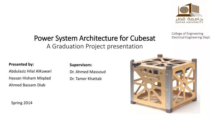
Power S ystem A rchitecture for Cubesat A Graduation Project presentation. College of Engineering Electrical Engineering Dept. Presented by: Abdulaziz Hilal AlKuwari Hassan Hisham Miqdad Ahmed Bassam Diab. Supervisors: Dr. Ahmed Massoud Dr. Tamer Khattab. Spring 2014.

E N D
Power System Architecture for CubesatA Graduation Project presentation College of EngineeringElectrical Engineering Dept. Presented by: AbdulazizHilal AlKuwari Hassan Hisham Miqdad Ahmed Bassam Diab Supervisors: Dr. Ahmed Massoud Dr. Tamer Khattab Spring 2014
Presentation overview • General Introduction About Cubesat. • Project Objectives. • System Divisions . • Time Schedule. • Simulation of QUbeSat Power System Architecture. • Test Results and Analysis • Modelling of the DC-DC Buck Converter. • Control of the DC-DC Buck Converter. • PV Model / Maximum-Power-Point-Tracking (MPPT). • Practical Implementation. • Project Cost • Future Work and Conclusion.
Literature Review • The satellite industry was only restricted to the space agencies and institutes till the first picosatellitewas created. • Cubesat design standards have been developed by the Joint cooperation of California Polytechnic State University (Cal Poly) at 1999. • Low Earth Orbit space missions. • Life span of about 9 months on an average.
Literature Review (cont’d) • General Cubesat standards and requirements
Why Cubesat? Universities develop Cubesat because of : • The fact that the components needed to have complete satellite system are already available on shelf with lower cost. • It is a standardized system which makes it simple to design the system and launch it.
Some Previous Cubesat Missions (cont’d) Number of successfully launched Cubesats versus the date of launching:
Mission of QU Satellite (QUbeSat) Qatar university Cubesat (QUbeSat) mission is to map and observe the current waste disposal sites in Qatar and search for the illegally disposed waste in the desert. gomspace.com
Project Objectives • The aim of the project is to designpower supply architecture for the (QUbeSat) that is responsible for feeding all the satellite subsystems. • The architecture is composed of different stages including power generation, storage and finally distribution.
Time Schedule The over all project life is three years!
Simulation Of QUbeSat Power System Architecture • The overall power system architecture of QUbeSat has been simulated using MATLAB/Simulink. • The system losses (hence efficiency) are assessed including non-idealities of the system components under different scenarios.
Simulation Of QUbeSat Power System Architecture(cont’d) Solar Arrays MPPT Converter Transfers the maximum power from the solar array which maximizes the system efficiency. • The five side of the satellite are connected in parallel. • Type of the PV panels is triple junction. gomspace.com
Simulation Of QUbeSat Power System Architecture(cont’d) Battery Pack Power Conditioning Converters Power condition converters step down/up the voltage of the battery to supply the satellite subsystems • Lithium-ion type. • Two connected in parallel having a rated capacity of total 1800 mAh and nominal voltage of 7.4V. gomspace.com
Simulation Of QUbeSat Power System Architecture(cont’d) • Open circuit voltage of the PV array is 5.38V. • Nominal voltage of the battery is 7.4V. • Aim of the MPPT-converter is to step up the PV array voltage to the battery level.
Simulation Of QUbeSat Power System Architecture(cont’d) The schematic of buck converter (including imperfections) The schematic of boost converter (including imperfections)
Simulation Of QUbeSat Power System Architecture (cont’d) • Three voltage levels to supply the loads. • The three converters simulated with the added imperfections. • The three converters are connected in parallel with the battery.
Simulation Of QUbeSat Power System Architecture(cont’d) • The design values (for QUbeSat)
Test Results and Analysis (cont’d) Case 1: • The power flow diagram below where the positive sign indicates loading and negative sign indicates supplying power
Test Results and Analysis (cont’d) Case 2: • The power flow diagram below where the positive sign indicates loading and negative sign indicates supplying power
Test Results and Analysis (cont’d) Case 3: • The power flow diagram below where the positive sign indicates loading and negative sign indicates supplying power
Modeling of the DC-DC Buck Converters • The step response of the converters shows large overshoot • Loads are sensitive to small voltage variations • The response can be improved closed loop control technique • An accurate model is needed to design the controller
Modeling of the DC-DC Buck Converters (cont’d) • The most significant imperfections that appears in the converter are: • The voltage drop across the diode. • The voltage drop across the switch. • The on-state resistance of the diode. • The on-state resistance of the switch. • The ESR of the Capacitor. • The internal resistance of the inductor.
Modeling of the DC-DC Buck Converters (cont’d) On-state Off-state
Modeling of the DC-DC Buck Converters (cont’d) • State space representation of the on-state mode of the buck converter • State space representation of the off-state mode of the buck converter
Modeling of the DC-DC Buck Converters (cont’d) • State Averaging • The switch is on at the time dT and off at the time (1-d)T. Thus the on-state and off state representations can be averaged as follow:
Modeling of the DC-DC Buck Converters (cont’d) • The Linearized Model of the Buck Converter
Modeling of the DC-DC Buck Converters (cont’d) • Result of the Buck DC- DC model Ideal Converter Derived Model Converter Physical Converter
Control of DC-DC Buck Converters • State Feedback Control
Control of DC-DC Buck Converters(Cont’d) • State Feedback Control with Integral Action
Control of DC-DC Buck Converters(Cont’d) The parameters used to simulate the converter The gain vector was calculated based on the following time domain specifications
PV Model • The aim of the PV model is to test the operation of the MPPT algorithm. • The available Practical PV Panel in the Lab is the 120W Polycrystalline BCT120-24. • The PV model chosen for the simulation is the Single-Diode general model.
PV Model (Cont’d) • The P-V characteristic curve of the Simulated Polycrystalline PV Panel for different solar insolation and temperature respectively.
Maximum-Power-Point-Tracking (MPPT) • MPPT can be achieved by different approaches and techniques, but the well-known and widely used algorithm is the Perturb & Observe (P & O) method because of: • Its simple implementation. • Reasonable convergence speed. • P & O technique can be well visualized in the figure shown in the next slide.
Maximum-Power-Point-Tracking (cont’d) • The (P&O) MPPT illustration is on Buck converter.
Maximum-Power-Point-Tracking (cont’d) • P&O method can be classified into: • Fixed perturb. • Adaptive perturb. • P&O with fixed perturb suffers some demerits and drawbacks: • Steady-state oscillations around the MPP due to fixed periodic tuning. • Possibility of tracking failure for rapid change of the atmospheric conditions especially the solar isolation. • The problem of steady-state oscillations can be minimized by applying small perturbation step-size, but results in slow down of the system.
Maximum-Power-Point-Tracking (cont’d) • Many researches went through improving the P&O method and make it adaptive-based by utilizing an automatic variable perturb tuning in order to satisfy: • Fast tracking response toward the maximum power point. • Low steady-state oscillations. • Can be achieved by applying a large perturb value at starting to reach the MPP fast, then minimize the perturb value to result in lower steady-state oscillations.
Maximum-Power-Point-Tracking (cont’d) • The simulation of the (P&O) algorithm has been performed on the available practical BCT120-24 PV panel to validate the functionality of the MPPT. • The converter used is Buck converter where its design parameters were chosen same as the practical design achieved in the lab.
Maximum-Power-Point-Tracking (cont’d) • PV module power for sudden change of solar insolation and fixed temperature (fixed-perturb of = 0.0001).
Maximum-Power-Point-Tracking (cont’d) • PV module power for sudden change of solar insolation and fixed temperature (adaptive-perturb of + (0.005 ×|dP/dV|)).
Practical Implementation • Converter Design Parameters.
Practical Implementation (cont’d) • State feedback Control on the 5V Buck converter • Open Loop Response