Download
1 / 22
220 likes | 368 Views
Bounding the strength of a Stochastic GW Background in LIGO’s S3 Data. Sukanta Bose (Washington State University, Pullman) for the LIGO Scientific Collaboration. LIGO DCC No. LIGO-G050536-00-D. SGWB: Properties. Individual detector strain: Zero mean Covariance: SGWB power

E N D
Bounding the strength of a Stochastic GW Background in LIGO’s S3 Data Sukanta Bose (Washington State University, Pullman) for the LIGO Scientific Collaboration LIGO DCC No. LIGO-G050536-00-D LSC/SB
SGWB: Properties • Individual detector strain: Zero mean • Covariance: • SGWB power spectrum: • What are we bounding? [Christensen, PRD46 (1992)] LSC/SB
The Search Statistic • Cross-correlation (CC) statistic: • Theoretical mean of CC statistic: • Theoretical variance: • Optimal filter: [Allen-Romano, PRD59, 102001 (1999)] LSC/SB
The Search Statistic (contd.) 60sec The optimal cross-correlation (CC) estimator is: i = 1 2 3 … t And the (inverse of the) optimal theoretical variance is: The measured Omega is: LSC/SB
S3: Reference sensitivities • The figure shows the typical equivalent-strain noise-densities of the 3 LIGO detectors during S3. Also shown is the strain density corresponding to a stochastic background with 50 100 500 Frequency (Hz) LSC/SB
Window & FFT Post-processing Analysis pipeline Detector 1 - 60 sec data segments Detector 2 - 60 sec data segments Software injections Downsample, HP filter, Freq-mask & calibrate Downsample, HP filter, Freq-mask & calibrate Estimate PSDs (using prev & next segs) Estimate PSDs (using prev & next segs) Compute optimal filter Qi and theoretical variance i2 Window & FFT Compute CC statistic Yi Optimally combine Yi , i2 LSC/SB
Choice of frequency cut-offs Overlap reduction functions Sensitivity vs Max cut-off for H1-H2 (S3) 0 50 100 150 200 250 300 Frequency (Hz) [Flanagan, PRD48, 2389 (1993)] Frequency bandwidth chosen from 70 - 220 Hz (H1-H2) 50 100 150 200 250 300 350 400 450 500 Max. cut-off frequency (Hz) LSC/SB
S3: H1-H2 Frequency mask LSC/SB
Sigma-cut of data intervals PI 60s t • Sigma-integrand is proportional to 1/(P1*P2) • P1, P2 estimated using data outside of 60s interval being analyzed, to avoid bias in cross-correlation • Not good PSD estimators when the noise is non-stationary over this time period • Compare this PSD to that computed with data in the interval; reject interval if they don’t agree LSC/SB
Sigma-cut of data intervals PI 60s t • Sigma-integrand is proportional to 1/(P1*P2) • P1, P2 estimated using data outside of 60s interval being analyzed, to avoid bias in cross-correlation • Not good PSD estimators when the noise is non-stationary over this time period • Compare this PSD to that computed with data in the interval; reject interval if they don’t agree LSC/SB
Distribution of the theoretical s (S2) S2 H1-L1 analysis: Distribution of the theoretical s LSC/SB
Distribution of the theoretical s (S3) S3 H1-H2 analysis: Distribution of the theoretical s S3 data was more non-stationary. LSC/SB
H1-L1 analysis: Long-duration features in CC-statistics (S2) S2 data was treated as “playground” for S3, esp., to check for long-duration trends. CC-statistic 5 15 25 35 45 Time (in days) LSC/SB
H1-L1 analysis: Lombe-Scargle Power Spectrum of CC statistics (S2) Injected line at 1/f = 1 hour Power 0 0.2 0.4 0.6 0.8 1 1.2 1.4 1.6 Frequency (in mHz) 1 day 10 min LSC/SB
H1-L1 analysis: Distribution of the Power of the CC-statistics (S2) 1000 N 1 0 2 4 6 8 10 12 Power LSC/SB
H1-L1 analysis: CC statistic trend (S2) PRELIMINARY LSC/SB
H1-L1 analysis(S2): Kolmogorov-Smirnov test Relative frequency -5 The K-S value of 0.483 implies that the distribution is close to normal. 0 -5 0 9 0 1 Relative freq. LSC/SB
S3 results: H1-H2 Error-estimate (+3s) plotted for the H1-H2 pair as a function of run time. LSC/SB
S3 results: H1-L1 Error-estimate (+3s) plotted for the H1-L1 pair as a function of run time. LSC/SB
PRELIMINARY LIGO results history on gw h1002 *[The LIGO Collaboration, PRD 69, 122004, (2004)] LSC/SB
Summary • The current best IFO-IFO upper-limit (published) is from S1: W < 23 (+/-4.6) • S2 bettered it to 0.018 (+0.007- 0.003) (PRELIMINARY) • The S3 studies are set to improve that • H1-H2 is the most sensitive pair, but it also suffers from cross-correlated terrestrial noise. H1-H2 coherence found weak in most frequency bands, except ~120Hz and ~180Hz; steps taken to excise these bands from analysis (in addition to frequency masking of certain lines). • The observed properties of the search statistics for the H1-H2 and H1-L1 pairs, after correcting for biases and known systematics, were found to closely fit the expected ones. • It now remains to run the search pipeline on the S3 science data to obtain upper-limits / confidence belts for a constant W. • Beyond current analysis: • Search for (f) ~ n(f/f0)n • Targeted searches LSC/SB
H1-L1 analysis: Long-duration features in CC-statistics (S2) S2 data was treated as “playground” for S3, esp., to check for long-duration trends. LSC/SB