Download
1 / 8
80 likes | 170 Views
Introduction. Visualization for Analyzing Trajectory-Based Metaheuristic Search Algorithms Steven HALIM 1 , Roland H.C. YAP 1 , and Hoong Chuin LAU 2 1 National University of Singapore, 2 Singapore Management University. Combinatorial Optimization Problems (COPs)

E N D
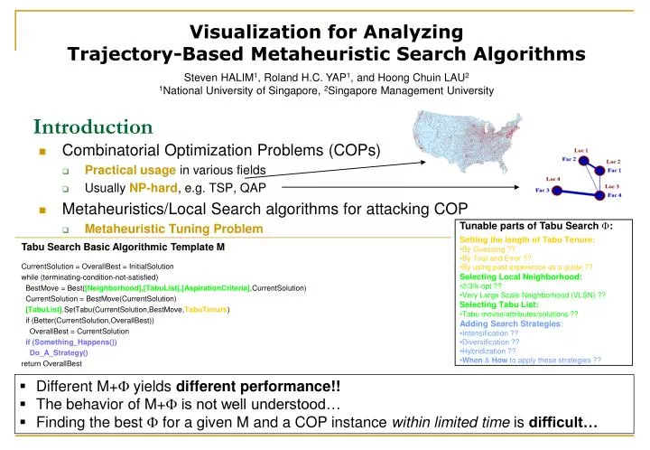
Introduction Visualization for Analyzing Trajectory-Based Metaheuristic Search Algorithms Steven HALIM1, Roland H.C. YAP1, and Hoong Chuin LAU21National University of Singapore, 2Singapore Management University • Combinatorial Optimization Problems (COPs) • Practical usage in various fields • Usually NP-hard, e.g. TSP, QAP • Metaheuristics/Local Search algorithms for attacking COP • Metaheuristic Tuning Problem • Tunable parts of Tabu Search : • Setting the length of Tabu Tenure: • By Guessing ?? • By Trial and Error ?? • By using past experience as a guide ?? • Selecting Local Neighborhood: • 2/3/k-opt ?? • Very Large Scale Neighborhood (VLSN) ?? • Selecting Tabu List: • Tabu moves/attributes/solutions ?? • Adding Search Strategies: • Intensification ?? • Diversification ?? • Hybridization ?? • When & How to apply these strategies ?? Tabu Search Basic Algorithmic Template M CurrentSolution = OverallBest = InitialSolution while (terminating-condition-not-satisfied) BestMove = Best([Neighborhood],[TabuList],[AspirationCriteria],CurrentSolution) CurrentSolution = BestMove(CurrentSolution) [TabuList].SetTabu(CurrentSolution,BestMove,TabuTenure) if (Better(CurrentSolution,OverallBest)) OverallBest = CurrentSolution if (Something_Happens()) Do_A_Strategy() return OverallBest • Different M+ yields different performance!! • The behavior of M+ is not well understood… • Finding the best for a given M and a COP instance within limited time is difficult…
Implement the metaheuristic Evaluate its performance Not good Good or give up Stop Modify the metaheuristic,usually ad hoc(“blind trial & error”) Approaches to Address Metaheuristic Tuning Problem • Common Practice:Ad Hoc (Blind) Tuning… • (Very) Slow • Emerging Trend: Various Tuning Methods • Black-Box --- Auto Configurator • CALIBRA (Adenso-Diaz & Laguna, 2006) • F-Race (Birattari, 2004), (Yuan & Gallagher, 2005), • +CARPS (Monett-Diaz, 2004) • White-Box --- Involving Human • Statistical Analysis (Jones & Forrest, 1995), (Fonlupt et al., 1997), (Merz, 2000), etc; • Human-Guided Search (Klau et al., 2002); • Visualization of Search (Syrjakow & Szczerbicka, 1999), (Kadluzdka et al., 2004) • Despite various approaches, there is still a need for a better solution for Tuning Problem!! Bottleneck !!!
Visual Diagnosis Tuning: Human + Computer Exploit humans! Olny srmat poelpe can raed tihs. cdnuolt blveiee taht I cluod aulaclty uesdnatnrd waht I was rdanieg. The phaonmneal pweor of the hmuan mnid, aoccdrnig to a rscheearch at Cmabrigde Uinervtisy, it deosn't mttaer in waht oredr the ltteers in a wrod are, the olny iprmoatnt tihng is taht the frist and lsat ltteer be in the rghit pclae. The rset can be a taotl mses and you can sitll raed it wouthit a porbelm. Tihs is bcuseae the huamn mnid deos not raed ervey lteter by istlef, but the wrod as a wlohe. Amzanig huh? yaeh and I awlyas tghuhot slpeling was ipmorantt! if you can raed tihs psas it on !! • Computer • Speed • Reliable • Endurance • Unbiased • Human • Intelligence • Visual Capability • Innovative • Common Sense Human is good in visualization!! *. Aware of crossings in TSP tour in a glance!! *. Reading distorted text!! *. Identifying similarities/patterns across seemingly disparate pictures. Bridging Interface: Visualization Task:Understanding and Tuningthe Local Search Task:Run Local Search andVisualize Search Information • How to understand the behavior of heuristic and stochastic local search??
Explaining Local Search Behavior There are several interesting questions about local search behavior: • Does it behave like as what we intended? • How good is the local search in intensification? • How good is the local search in diversification? • Is there any sign of cycling behavior? • How does the local search algorithm make progress? • Where in the search space does the search spend most of its time? • What is the effect of modifying a certain search parameter/component/strategy w.r.t the search behavior? • How far is the starting (initial) solution to the global optima/best found solution? • Does the search quickly find the global optima/best found solution region or does it wander around in other regions? • How wide is the local search coverage? • How do two different algorithms compare? • Advantages for understanding local search behavior: • Better equipped for addressing the Tuning Problem • Can spot and debug the incorrect behavior • Improving the underlying local search algorithm. Existing approaches for explaining Local Search behavior: • Objective Value/Solution Quality/Robustness • Run Time/Length Distribution [Hoos, 1998] • Fitness Distance Correlation [Jones, 1995] • Problem Specific, e.g. TSP [Klau et al., 2002] • N-to-2-Space Mapping [Kadluczka, 2004] • 2-D Animation [Syrjakow & Szczerbicka, 1999] • Search TrajectoryVisualization [this work]
Search Trajectory Visualization – Main Concepts • Analogy: Mountainous Landscape ~ Fitness Landscape of an instance of combinatorial optimization problem. • Objective: Explaining the local search trajectory using anchor points, distance metric and fitness function!! 1. Without anchor points, the behavior of the pink trajectory is hard to be explained. 2. Do several local search runs with different configurations, record diverse local optima/anchor points (circled). 3. With anchor points, the behavior of the pink trajectory is as follows: trapped in region that contains red/blue anchor points, thus failed to visit good solutions, the green/orange anchor points. 4. The behavior of thepale blue trajectory is as follows: after reaching a local optima, it diversifies to another place. It manages to reach green and orange anchor points, and thus its performance is better than the pink trajectory in Figure 3.
Laying Out Points in Abstract 2-D Space • Search Trajectory Visualization • In Practice • Layout the points in Abstract 2-D Space • Points that are close in N-dimensional space in terms of distance metric (hamming, permutation distance, etc)are laid out close to each other in the abstract 2-D space and vice versa. • This utilizes human strength in discerning 2-D spatial information. • Layout First Phase: • The anchor points are measured with each other using distance metric. • The anchor points are installed greedily in abstract 2-D space • Re-optimize using the Spring Model layout algorithm. • Layout Second Phase: • Again, using Spring Model algorithm, the points along search trajectory are aid out in abstract 2-D space using these anchor points as reference. • Presentation Aspects: • Color coding is used to enhance our understanding: blue: good, green: medium, brown: pooranchor points. • The search trajectory is animated over time. Anchor Points are quite close to each other. Trapped in cycling near Anchor Point C Only covers regions near Anchor Point D and E Anchor Points are quite close to each other, but their quality are different. Trapped in cycling near Anchor Point C because it is attractive (green) Only covers regions near Anchor Point D and E, which are good regions (blue and green)
Viz: Local Search Visual Analysis Suite • Features: • Can answer all questions of local search behavior shown previously • Multi Visualization • Animation • Color & Highlighting • Visual Comparison • Customize-able GUI • Off-line Analysis Tools: • Analyze Local Search RunLogs • Technologies used: • Visual C#.NET 2005 • .NET Framework 2.0 • OpenGL/CsGL
A TSP Example Explaining 2 Iterated Local Search (ILS) performance and behavior for Traveling Salesman Problem (TSP)!! Fitness Distance Correlation analysis confirmed the presence of `Big Valley’: the distance of most local optima w.r.t best found are only 1/4 of the diameter and the FDC coefficient is high. Objective Value chart: In overall, ILS_A (red) seems to find better solutions than ILS_B (blue). Eventually, the best solution found by ILS_A is better than ILS_B. TSP Fitness Landscape: `Big Valley’ (circled) - a cluster of good anchor points (blue) are located in the middle of the screen and are close to each other… After filtering the points above 7.5%-off from best found value, ILS_A (red) covers a lot more good points, which are near to the `Big Valley’ (center of the screen) than ILS_B (blue). When the search trajectory is played back iteratively, the trajectory of ILS_A (red) is concentrated in the region near `Big Valley’ whereas the trajectory of ILS_B (blue) is more erratic. Conclusion: Viz can be used to explain local search behaviors,which is a necessary step before tuning the local search algorithm. For more details, please visit: http://www.comp.nus.edu.sg/~stevenha/viz