Accelerating MATLAB with CUDA
Accelerating MATLAB with CUDA. Won-Ki Jeong University of Utah wkjeong@cs.utah.edu. Massimiliano Fatica NVIDIA mfatica@nvidia.com. Overview.

Accelerating MATLAB with CUDA
E N D
Presentation Transcript
Accelerating MATLAB with CUDA Won-Ki Jeong University of Utah wkjeong@cs.utah.edu Massimiliano Fatica NVIDIA mfatica@nvidia.com
Overview MATLAB can be easily extended via MEX files to take advantage of the computational power offered by the latest NVIDIA GPUs (GeForce 8800, Quadro FX5600, Tesla). Programming the GPU for computational purposes was a very cumbersome task before CUDA. Using CUDA, it is now very easy to achieve impressive speed-up with minimal effort. This work is a proof of concept that shows the feasibility and benefits of using this approach.
MEX file • Even though MATLAB is built on many well-optimized libraries, some functions can perform better when written in a compiled language (e.g. C and Fortran). • MATLAB provides a convenient API for interfacing code written in C and FORTRAN to MATLAB functions with MEX files. • MEX files could be used to exploit multi-core processors with OpenMP or threaded codes or like in this case to offload functions to the GPU.
NVMEX • Native MATLAB script cannot parse CUDA code • New MATLAB script nvmex.m compiles CUDA code (.cu) to create MATLAB function files • Syntax similar to original mex script: >> nvmex –f nvmexopts.bat filename.cu –IC:\cuda\include –LC:\cuda\lib -lcudart Available for Windows and Linux from: http://developer.nvidia.com/object/matlab_cuda.html
Mex files for CUDA A typical mex file will perform the following steps: • Convert from double to single precision • Rearrange the data layout for complex data • Allocate memory on the GPU • Transfer the data from the host to the GPU • Perform computation on GPU (library, custom code) • Transfer results from the GPU to the host • Rearrange the data layout for complex data • Convert from single to double • Clean up memory and return results to MATLAB Some of these steps will go away with new versions of the library (2,7) and new hardware (1,8)
CUDA MEX example Additional code in MEX file to handle CUDA /*Parse input, convert to single precision and to interleaved complex format */ ….. /* Allocate array on the GPU */ cufftComplex *rhs_complex_d; cudaMalloc( (void **) &rhs_complex_d,sizeof(cufftComplex)*N*M); /* Copy input array in interleaved format to the GPU */ cudaMemcpy( rhs_complex_d, input_single, sizeof(cufftComplex)*N*M, cudaMemcpyHostToDevice); /* Create plan for CUDA FFT NB: transposing dimensions*/ cufftPlan2d(&plan, N, M, CUFFT_C2C) ; /* Execute FFT on GPU */ cufftExecC2C(plan, rhs_complex_d, rhs_complex_d, CUFFT_INVERSE) ; /* Copy result back to host */ cudaMemcpy( input_single, rhs_complex_d, sizeof(cufftComplex)*N*M, cudaMemcpyDeviceToHost); /* Clean up memory and plan on the GPU */ cufftDestroy(plan); cudaFree(rhs_complex_d); /*Convert back to double precision and to split complex format */ ….
Initial study • Focus on 2D FFTs. • FFT-based methods are often used in single precision ( for example in image processing ) • Mex files to overload MATLAB functions, no modification between the original MATLAB code and the accelerated one. • Application selected for this study: solution of the Euler equations in vorticity form using a pseudo-spectral method.
Implementation details: Case A) FFT2.mex and IFFT2.mex Mex file in C with CUDA FFT functions. Standard mex script could be used. Overall effort: few hours Case B) Szeta.mex: Vorticity source term written in CUDA Mex file in CUDA with calls to CUDA FFT functions. Small modifications necessary to handle files with a .cu suffix Overall effort: ½ hour (starting from working mex file for 2D FFT)
Configuration Hardware: AMD Opteron 250 with 4 GB of memory NVIDIA GeForce 8800 GTX Software: Windows XP and Microsoft VC8 compiler RedHat Enterprise Linux 4 32 bit, gcc compiler MATLAB R2006b CUDA 1.0
Vorticity source term http://www.amath.washington.edu/courses/571-winter-2006/matlab/Szeta.m function S = Szeta(zeta,k,nu4) % Pseudospectral calculation of vorticity source term % S = -(- psi_y*zeta_x + psi_x*zeta_y) + nu4*del^4 zeta % on a square periodic domain, where zeta = psi_xx + psi_yy is an NxN matrix % of vorticity and k is vector of Fourier wavenumbers in each direction. % Output is an NxN matrix of S at all pseudospectral gridpoints zetahat = fft2(zeta); [KX KY] = meshgrid(k,k); % Matrix of (x,y) wavenumbers corresponding % to Fourier mode (m,n) del2 = -(KX.^2 + KY.^2); del2(1,1) = 1; % Set to nonzero to avoid division by zero when inverting % Laplacian to get psi psihat = zetahat./del2; dpsidx = real(ifft2(1i*KX.*psihat)); dpsidy = real(ifft2(1i*KY.*psihat)); dzetadx = real(ifft2(1i*KX.*zetahat)); dzetady = real(ifft2(1i*KY.*zetahat)); diff4 = real(ifft2(del2.^2.*zetahat)); S = -(-dpsidy.*dzetadx + dpsidx.*dzetady) - nu4*diff4;
Caveats The current CUDA FFT library only supports interleaved format for complex data while MATLAB stores all the real data followed by the imaginary data. Complex to complex (C2C) transforms used The accelerated computations are not taking advantage of the symmetry of the transforms. The current GPU hardware only supports single precision (double precision will be available in the next generation GPU towards the end of the year). Conversion to/from single from/to double is consuming a significant portion of wall clock time.
Advection of an elliptic vortex 256x256 mesh, 512 RK4 steps, Linux, MATLAB file http://www.amath.washington.edu/courses/571-winter-2006/matlab/FS_vortex.m MATLAB 168 seconds MATLAB with CUDA (single precision FFTs) 14.9 seconds (11x)
Pseudo-spectral simulation of 2D Isotropic turbulence. 512x512 mesh, 400 RK4 steps, Windows XP, MATLAB file http://www.amath.washington.edu/courses/571-winter-2006/matlab/FS_2Dturb.m MATLAB 992 seconds MATLAB with CUDA (single precision FFTs) 93 seconds
Power spectrum of vorticity is very sensitive to fine scales. Result from original MATLAB run and CUDA accelerated one are in excellent agreement MATLAB run CUDA accelerated MATLAB run
Timing details 1024x1024 mesh, 400 RK4 steps on Windows, 2D isotropic turbulence
Conclusion • Integration of CUDA is straightforward as a MEX plug-in • No need for users to leave MATLAB to run big simulations: high productivity • Relevant speed-ups even for small size grids • Plenty of opportunities for further optimizations