STAT131 Week 7 L1b Exponential Distribution & relationship to Poisson

STAT131Week 7 L1b Exponential Distribution & relationship to Poisson by Anne Porter alp@uow.edu.au

Exponential distribution • The Poisson distribution may involve the count of events in a given time period. • Looking at this differently we can measure • The time until the first event occurs and because • the exponential process has no memory of the previous event • The time until the next event or • The time between events.

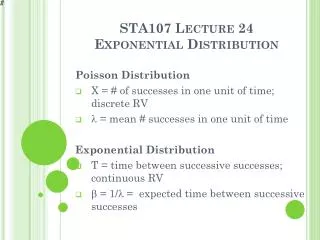
Exponential Process • If we have a homogeneous Poisson process with a rate of events  per unit of time, then the time from t=0 to the first event is a random variable with an exponential distribution. We will symbolise this random variable as Y. As with the Poisson it will have the parameter  . • There are other ways in which the exponential can arise

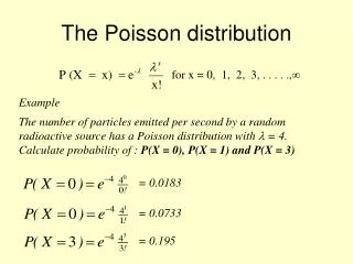
Probability: Poisson • Let the number of events between time zero and time t be denoted as X occurring with a rate of events . Then the discrete random variable X has a . The probability that there are no events between time zero and time t is Poisson distribution calculated using the Poisson distribution function Function key on calculator

Probability: Poisson • Let the number of events between time zero and time t be denoted as Xt occurring with a rate of events . Then the discrete random variable Xt has a . The probability that there are no events between time zero and time t is Poisson distribution calculated using the Poisson distribution function

Poisson link to the Exponential No events between time zero and time t Is the same as The time of the first event is greater than t

Poisson link to the Exponential One or more between time zero and time t Is the same as The time of the first event is less than t The Cumulative Distribution function F(Y) is P(Y<y) and that is equal to 1-e-lt

f(y) F(y) 1 l 0 y 0 y Link from probability density function (pdf) to the cumulative distribution function (cdf) f(y)=e-t F(y)=1-e-t How do we get f(y) from F(y)? By differentiating ie

Probability: Exponential To find the probability of a continuous Random Variable X taking on some value between a and b is given by: The function for the exponential is: Hence we have the probability of Y taking a value between a and b is: Easier ...

= Probability:Exponential = The probability that the random event Y takes on a value between time1 and time 2 is given by

Features of the Exponential distribution (i) What is the shape of the distribution and associated questions as to what is the probability of some event happening? (ii) What is the centre of the distribution? (iii) What is the spread of the distribution? (iv) How do we calibrate the model given a set of data? (v) Does the model fit the data?

Centre:Exponential • The mean of the Random Variable Y is given as for all the continuous distributions by • ie in this instance substituting the function for the exponential • This is equivalent to

Spread: Variance • The general form to find the variance is • or • or • We will make use of the following algebraically equivalent property of the exponential EASY APPROACH

Spread: Standard deviation • The standard deviation of the random variable Y is the • The standard deviation of the exponential is the same as the mean

Calibration of the Exponential Model • To estimate  based on a sample we set the mean of the distribution equal to the sample mean that is so

Assessment of model fit • Charts -histogram compared to probability density function • Simulation, comparing • histograms • plots simulated from a model with that rate and of same size.

Goodness of fit • If then the data fit the model • Informal if there is evidence of lack of fit • Formal if > tabulated value for a given level of a (we will use 0.05) and df=g-p-1

Assumptions: Goodness of fit • The expected number in each cell or bin should be > 5. If they are not adjacent cells should be combined.

An example: Exponential • A sugar refinery has three processing plants, all of which receive raw sugar in bulk. The amount of sugar that one plant can process in one day can be modelled as having an exponential distribution with a mean of 4 (measurements in tons) for each of the three plants. (a) What is the probability that the plant will process exactly four tons on a randomly selected day? The probability of exactly equally some constant is zero for any continuous distribution.

An example: Exponential • A sugar refinery has three processing plants, all of which receive raw sugar in bulk. The amount of sugar that one plant can process in one day can be modelled as having an exponential distribution with a mean of 4 (measurements in tons) for each of the three plants. (b) What is the probability that a plant will process more than four tons on a given day. 1- P(0<Y<4) How do we find the probability of there being between 0 and 4 tons?

An example: Exponential • A sugar refinery has three processing plants, all of which receive raw sugar in bulk. The amount of sugar that one plant can process in one day can be modelled as having an exponential distribution with a mean of 4 (measurements in tons) for each of the three plants. (b) What is the probability that a plant will process more than four tons on a given day. 1- P(0<Y<4) P(0<Y<4) = What is the dimension t in this example? tons What is t1 and t2 ? 0 and 4 How do we calibrate the rate l?

An example: Exponential • A sugar refinery has three processing plants, all of which receive raw sugar in bulk. The amount of sugar that one plant can process in one day can be modelled as having an exponential distribution with a mean of 4 (measurements in tons) for each of the three plants. (b) What is the probability that a plant will process more than four tons on a given day. 1- P(0<Y<4) What is the dimension t in this example? tons What is t1 and t2 ? 0 and 4 How do we calibrate the rate l?

P(0<Y<4) An example: Exponential • A sugar refinery has three processing plants, all of which receive raw sugar in bulk. The amount of sugar that one plant can process in one day can be modelled as having an exponential distribution with a mean of 4 (measurements in tons) for each of the three plants. (b) What is the probability that a plant will process more than four tons on a given day. 1-P(0<Y<4) =1-0.6321=0.3679 =e0-e-1 =1-0.3679 =0.6321

An example: picking the model • A sugar refinery has three processing plants, all of which receive raw sugar in bulk. The amount of sugar that one plant can process in one day can be modelled as having an exponential distribution with a mean of 4 (measurements in tons) for each of the three plants. (c) If the plants (see problem 4) operate independently, find the probability that exactly three of the plants will process more than 4 tons on a given day.

What do we do if the data does not fit the model? • If the model does not fit, ask 'why not?' Could it be that one or more assumptions do not hold. • Look at changes over time, rate or lack of independence in time periods • Examine which cells have the largest lack of fit • Look at theoretical relationships eg mean=variance or mean=standard deviation where they exist

Current summary:General Discrete; Binomial, Poisson, General continuous: Normal, Exponential • Context or assumptions relating to problems • shape (probability) • Centre, spread • Outliers, patterns • Calibration of model • Using statistics from samples • Does the data fit a model • Charts,2GOF ,simulation

Current summary: Discrete Vs Continuous Models • For students to complete

STAT131 Week 7 L1b Exponential Distribution & relationship to Poisson