Download
1 / 39
400 likes | 555 Views
MPEG 4 Structured Audio:. Algorithmic Sound for the Internet and Beyond. John Lazzaro John Wawrzynek Sep 1, 1999. CS Division University of California at Berkeley www.cs.berkeley.edu/~johnw. MPEG 4 Structured Audio. Outline: Motivation for structured audio Introduction to MP4-SA

E N D
MPEG 4 Structured Audio: Algorithmic Sound for the Internet and Beyond John Lazzaro John Wawrzynek Sep 1, 1999 CS Division University of California at Berkeley www.cs.berkeley.edu/~johnw
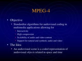
MPEG 4 Structured Audio Outline: • Motivation for structured audio • Introduction to MP4-SA • Example encoding • C translator • Physical Instrument Modeling • Hardware Architectures • Future directions
Digital Audio Basics amp 16-bit samples time 44.1kHz sample rate encoder Traditional Compression: decoder • How well does this work? • True Lossless: 2.5X reduction • Shorten, T. Robinson (Cambridge University) • “Perceptually Lossless” : 10X-20X reduction • MP3, Dolby AC3, … • mono: 705.6 kbps • Cell-phone network: 5-10kbps • dialup modems: 50 kpbs • xDSL: 128 to 1000 kbps
The Kolmogorov alternative: • Write acomputer program that generates the desired audio stream. • Transmit the computer program. • To decode, execute the program. Similar to Postscript! • MPEG-4 Structured Audio (MP4-SA) uses this approach. • Final draft standard: Nov 15, 1998. • Eric Schierer, Editor (MIT Media Lab). • http://sound.media.mit.edu/~eds/mpeg4/
MP4-SA Encoding MP4-SA Decoders • are interpreters or compilers. • may be a creative act: writing a program. • directly (emacs), or • indirectly (GUI, webpage) • In this case, MP4-SA is a lossless compressor. • may be automatic -- given a sound, an encoder writes a program that generates the sound. • Automatic encoding is a hard problem in the general case.
Key Application: Music Production Network MP4-SA Maps to Modern Music Production Premium on low-bandwidth • “The Program” • synthesis algorithms • effects “boxes” • mixers • “The Decoder” • sound rendering Musical performance Mix-down control information • Modern Music Production is Computer based. • Musicians enter performances into computers as control information, not audio waveforms. • Digital synthesizers, effects, and mixes create the final audio, under engineer/producer control.
Key Application: Music Production MP4-SA Maps to Modern Music Production • “The Program” • synthesis algorithms • effects “boxes” • mixers Standard Framework • “The Decoder” • sound rendering Musical performance Mix-down control information File System • Modern Music Production is Computer based. • Musicians enter performances into computers as control information, not audio waveforms. • Digital synthesizers, effects, and mixes create the final audio, under engineer/producer control. Ideal format for collaborative productions, remixes, ...
MPEG 4 Structured Audio: • A binary file format that encodes: • The programming language SAOL (say: sail). • The musical score language SASL. • Legacy support for MIDI. • Audio sample data. • Result is normative: an MP4-SA file will sound identical on all compliant decoders. • Different from MIDI files.
MPEG 4 Standard MPEG 4 video audio system Natural coding Synthetic coding SA TTS AAC T/F CELP Parametric Structured Audio: One “component” in the MPEG audio standard. ISO/IEC 14496-3 sec5
MPEG 4 Standard MPEG 4 video audio system Natural coding Synthetic coding SA TTS AAC T/F CELP Parametric Advanced Audio Coding: successor to MP3, delivers highest quality audio, and highest bit-rate.
MPEG 4 Standard MPEG 4 video audio system Natural coding Synthetic coding SA TTS AAC T/F CELP Parametric Time-Frequency Coding: Meant for a moderate bit/sec range, with moderate quality.
MPEG 4 Standard MPEG 4 video audio system Natural coding Synthetic coding SA TTS AAC T/F CELP Parametric Code Excited Linear Prediction: Low bit rate coder, works best as a speech coder.
MPEG 4 Standard MPEG 4 video audio system Natural coding Synthetic coding SA TTS AAC T/F CELP Parametric Parametric coders: Very-low bit rate coder, works best as as a speech coder.
MPEG 4 Standard MPEG 4 video audio system Natural coding Synthetic coding SA TTS AAC T/F CELP Parametric Text-to-Speech: Takes phonetic and prosadic control information, produces syntesized speech.
MPEG 4 Standard MPEG 4 video audio system Natural coding Synthetic coding SA TTS AAC T/F CELP Parametric “System” level includes mechanisms for composing and synchronizing audio (& video) components.
Why SAOL and MP4-SA?Why not Java? Amplitude & timbre envelopes: 10’s of msec Sample-by-sample 10’s of usec Note-by-note: 100’s of msec • Musical performance have temporal structure that changes over several timescales: • Writing sound generation code in a conventional language results in code dominated by time-scale management. • Hard to maintain, hard to optimize.
Time management is built into SAOL. • A SAOL program executes by moving a simulated clock forward in time, performing calculations along the way in a synchronous fashion. • Work is scheduled to happen: • at the a-rate (the audio sample rate) • at the k-rate (envelope control rate) • at the i-rate (rate for new notes) • Language variables are typed as a/k/i-rate. • A language statement is scheduled based on the rate of the variables it contains.
SAOL, SASL, and Scheduling: • Sound creation in MP4-SA can be compared to a musician playing notes on an instrument. • A SAOL subprogram (called an instr or instrument) serves as the instrument. • SASL commands (called score lines) act to play notes on SAOL instruments. • Many instances of a SAOL instr can be active at one time, making sounds corresponding to notes launched by different score lines in a SASL file.
SAOL Instruments ... Contains all the instructions for playing a note: -- Code that runs at note launch. (once per i-pass) -- Code that models timbre evolution at the k-rate. (once per kpass) -- Code to generate audio samples at the a-rate. (once per a-pass) Single Note Execution Trace Executing a Note … (k-rate: 4 kHz, a-rate: 40 kHz) time(us) pass 0 i-pass 0 k-pass 0 a-pass 25 a-pass 50 a-pass ... 225 a-pass 250 k-pass 250 a-pass 275 a-pass 300 a-pass ... 475 a-pass 500 k-pass 500 a-pass 525 a-pass ...
An example: • This SASL file plays melody on tone: 0.5 tone 0.75 52 0.25 1.5 tone 0.75 64 0.25 2.5 tone 0.5 63 0.25 3 tone 0.25 59 0.2 3.25 tone 0.25 61 0.225 3.5 tone 0.5 63 0.225 4 tone 0.5 64 0.25 5 end When instance is launched Instance parameters (note number, loudness) How long instrument runs • SAOL instrument tone, that plays a gated sine wave. (SAOL code in next slide.)
SAOL code for tone instr tone (note, loudness) { ivar a; // sets osc f ksig env; // env output asig x, y; // osc state asig init; a = 2*sin(3.141597*cpsmidi(note)/s_rate); env = kline(0, 0.1, 0.5, dur-0.2, 0.5, 0.1, 0); if (init == 0) // first a-pass only { x = loudness; init = 1; } x = x - a*y; // the FLOPS happen in y = y + a*x; // these 3 statements output(y*env); // creates audio output } // end of instr tone
SAOL code for tone instr tone (note, loudness) { ivar a; // sets osc f ksig env; // env output asig x, y; // osc state asig init; a = 2*sin(3.141597*cpsmidi(note)/s_rate); env = kline(0, 0.1, 0.5, dur-0.2, 0.5, 0.1, 0); if (init == 0) // first a-pass only { x = loudness; init = 1; } x = x - a*y; // the FLOPS happen in y = y + a*x; // these 3 statements output(y*env); // creates audio output } // end of instr tone i-rate
SAOL code for tone instr tone (note, loudness) { ivar a; // sets osc f ksig env; // env output asig x, y; // osc state asig init; a = 2*sin(3.141597*cpsmidi(note)/s_rate); env = kline(0, 0.1, 0.5, dur-0.2, 0.5, 0.1, 0); if (init == 0) // first a-pass only { x = loudness; init = 1; } x = x - a*y; // the FLOPS happen in y = y + a*x; // these 3 statements output(y*env); // creates audio output } // end of instr tone k-rate
SAOL code for tone instr tone (note, loudness) { ivar a; // sets osc f ksig env; // env output asig x, y; // osc state asig init; a = 2*sin(3.141597*cpsmidi(note)/s_rate); env = kline(0, 0.1, 0.5, dur-0.2, 0.5, 0.1, 0); if (init == 0) // first a-pass only { x = loudness; init = 1; } x = x - a*y; // the FLOPS happen in y = y + a*x; // these 3 statements output(y*env); // creates audio output } // end of instr tone a-rate
SAOL: Unique Features • Rate semantics: • i/k/a-rate execution • Vector arithmetic: • ex: A=B+Cfor i=1,n A[i]=B[i]+C[i] • All floating-point arithmetic. • Extensive build-in audio function library: • signal generators, table operators, pitch converters, filters, fft, sample rate conversion, effects, ...
SAOL: Unique Features B A bus C D • Instrument communication through bus structures: • Dynamic instrument creation and control. • Scheduler and language support for MIDI and SASL scores.
Sfront - a SAOL-to-C translator sfront foo.mp4 sa.c • Handles SAOL, SASL, MIDI, uncompressed samples. SAOL SASL foo.mp4 sfront MIDI sa.c Uncompressed samples • Converts MP4-SA files to a C program, that when executed, produces audio. • Runs on UNIX, Win98/NT. • Licensed under the GNU public license (GPL). • www.cs.berkeley.edu/~lazzaro/sa
Sfront Benchmarks Sfront version 0.36 Machine: 450 Mhz Pentium III, 128 MB, gcc version egcs-2.91.66, -O3 optimizer Audio sample rate: 44.1 kHz for all examples MP3 compression ratio = 11
Sfront Performance Summary: • Rendering (file decoding): • Current performance: a benchmark suite of moderately complex MP4-SA streams computes in a time equivalent to the audio it generates, on a 400 Mhz Ultrasparc & 450 Mhz Pentium. • Real-time interaction: • with a MIDI keyboard with acceptable latency (~20 ms) and microphone input.
Interesting Issues: • MP4-SA puts emphasis on sound synthesis methods that can be described in a small amount of space. • Physical Modeling good • Sampling Natural Instruments bad • If models are chosen carefully, compression ratios of 100 to 10,000 are possible. • Physical Modeling is relatively immature, but holds much promise.
Struck/Plucked Instrument Model attack section linear modes (resonances) M1 Aluminum Bar Sounds M2 single strike M3 output striker multiple strikes Mn amplitude Digital resonator: Yn = Yn-1 + Yn-2 + Xn frequency Examples: struck bars, bells, drums, plucked strings Parameters: striker characteristics, resonator constants
Blown Instrument Model jet Blown Pipe Sounds non-linear element linear element (resonant modes) x y excitation tube amplitude y brass pipe x overblown frequency Examples: pipes, flutes, etc. Parameters: shape of non-linear function, resonator constants
Physical Modeling Summary • Models instrument not sound. • Advantages over traditional synthesis techniques (FM, sample-based): • Compact descriptions. • Physical parameterization leads to: • more intuitive control • lower control bandwidth • State accurate simulation leads to: • efficiency in re-excitation • emulation of otherwise missing effects • Ultimately - more realistic sounds.
Physical Modeling Summary (cont.) • Disadvantages: • potential for high computational complexity • Approaches: • PDE (partial differential equation) approach would be nice, but probably not practical. • ODE (ordinary differential equation, lumped circuit models) practical and very general. Capture essential physics. • Wave-guide filters provide a more efficient alternative in some cases.
Interesting Issues (cont.): • MP4-SA specifies that a decoder produces audio that “sounds identical” to computing the program accurately. • A new role for psychophysics: Instead of using psychophysics to squeeze bits out of a sound representation, MP4-SA decoders will use psychophysics to squeeze FLOPS out of sound computations. • Leverage spectral and temporal masking.
Interesting Issues (cont.): • MP4-SA can be used in a way similar to traditional compression except that the compression method can be ad hoc: • Frame-work for experimentation in encoding. • Hope for automatic encoding, if done in a voice specific way: • vocals • guitar • sax • and other hard-to-synthesize sounds.
Running SAOL on Conventional Architectures • Lessons Learned from SAOL development: • Temporal typing of variables has the nice side effect of marking the inner loops. • Typically, a-rate = 10X to 100X k-rate • A-rate code optimization : moving subexpressions into k-rate or i-rate. • SAOL semantics support a static heap. • No recursion, all variables sp floats, no pointers ... simplifies optimization. • Other researchers (Giorgio Zoia - ETH) focusing on blocking all a-passes for an instance, reducing overhead. • Processors with SIMD FP support (Intel SSE, AMD 3DNow!) will be a good match.
Fixed-Function Hardware for SAOL Accelerators • Unlike MPEG-2 chips, DVD chips, etc., its not clear how MP4-SA can be accelerated by rolling an ASIC. • Since every MP4-SA file is a new algorithm. • Common opcodes can be hardwired and the general characteristics of typical MP4-SA files could be leveraged to specialize a conventional processor design. • But the language is only six months old; execution frequencies are not known. • Reconfigurable computing architectures might hold promise (however, MP4-SA is all floating point).
Directions / Research Opportunities • Compiler optimizations for: • SAOL and other languages with rate semantics • high-performance SIMD architectures • runtime code specialization • Runtime scheduling under limited compute resources. • SAOL programming environments. • Physical modeling. • Automatic encoding.