Inventory Costs
Inventory Costs. Interest or Opportunity Costs Storage and Handling Costs Taxes, Insurance, and Shrinkage Costs Ordering and Setup Costs Transportation Costs. Cycle Inventory Safety Stock Inventory Anticipation Inventory Pipeline Inventory. Q + 0 2. Average cycle inventory =

Inventory Costs
E N D
Presentation Transcript
Inventory Costs • Interest or Opportunity Costs • Storage and Handling Costs • Taxes, Insurance, and Shrinkage Costs • Ordering and Setup Costs • Transportation Costs
Cycle Inventory Safety Stock Inventory Anticipation Inventory Pipeline Inventory Q + 0 2 Average cycle inventory = Pipeline inventory = DL = dL Types of Inventory
Class C 100 — 90 — 80 — 70 — 60 — 50 — 40 — 30 — 20 — 10 — 0 — Class B Class A Percentage of dollar value 10 20 30 40 50 60 70 80 90 100 Percentage of items ABC Analysis Figure 10.1
Assumptions Economic Order Quantity Demand rate is constant No constraints on lot size Only relevant costs are holding and ordering/setup Decisions for items are independent from other items No uncertainty in lead time or supply
Receive order Inventory depletion (demand rate) Q Q — 2 On-hand inventory (units) Average cycle inventory 1 cycle Time Economic Order Quantity Figure 10.2
Current cost 3000 — 2000 — 1000 — 0 — Q 2 D Q Total cost = (H) + (S) Annual cost (dollars) Q 2 Holding cost = (H) D Q Ordering cost = (S) | | | | | | | | 50 100 150 200 250 300 350 400 Current Q Lot Size (Q) Economic Order Quantity
Current cost 3000 — 2000 — 1000 — 0 — Bird feeder costs Q 2 D Q D = (18 /week)(52 weeks) = 936 units H = 0.25 ($60/unit) = $15 S = $45 Q = 75 units Total cost = (H) + (S) Annual cost (dollars) Q 2 Holding cost = (H) Q 2 D Q 2DS H C = (H) + (S) EOQ = C = $562 + $562 = $1124 D Q Ordering cost = (S) Lowest cost | | | | | | | | 50 100 150 200 250 300 350 400 Current Q Best Q (EOQ) Lot Size (Q) Example 10.1 Economic Order Quantity
Current cost 3000 — 2000 — 1000 — 0 — Birdfeeder costs Time between orders Q 2 D Q D = (18 /week)(52 weeks) = 936 units H = 0.25 ($60/unit) = $15 S = $45 Q = 75 units Total cost = (H) + (S) EOQ D TBOEOQ = = 75/936 = 0.080 year TBOEOQ = (75/936)(12) = 0.96 months TBOEOQ = (75/936)(52) = 4.17 weeks TBOEOQ = (75/936)(365) = 29.25 days Annual cost (dollars) Lowest cost | | | | | | | | 50 100 150 200 250 300 350 400 Current Q Best Q (EOQ) Lot Size (Q) Example 10.1 Economic Order Quantity
IP IP Order received Order received Order received Order received Q Q Q OH On-hand inventory R Order placed Order placed Order placed Time L1 L2 L3 TBO1 TBO2 TBO3 Figure 10.7 Uncertain Demand
Cycle-service level = 85% Probability of stockout (1.0 – 0.85 = 0.15) Average demand during lead time R zL Reorder Point / Safety Stock Figure 10.8
st = 15 st = 15 st = 15 st = 26 + 75 Demand for week 1 + sL = st L = 5 2 = 7.1 225 Demand for three-week lead time 75 Demand for week 2 = Example 10.3 75 Demand for week 3 Lead Time Distributions Bird feeder Lead Time Distribution t = 1 week d = 18 L = 2 Safety stock = zsL = 1.28(7.1) = 9.1 or 9 units Reorder point = dL + Safety stock = 2(18) + 9 = 45 units
st = 15 st = 15 st = 15 st = 26 + 75 Demand for week 1 + 75 2 936 75 C = ($15) + ($45) + 9($15) 225 Demand for three-week lead time 75 Demand for week 2 = Example 10.3 75 Demand for week 3 Lead Time Distributions Bird feeder Lead Time Distribution t = 1 week d = 18 L = 2 Reorder point = 2(18) + 9 = 45 units C = $562.50 + $561.60 + $135 = $1259.10
T IP IP IP Order received Order received Order received Q3 Q1 OH OH Q2 IP1 IP3 IP2 On-hand inventory Order placed Order placed L L L Time P P Protection interval Periodic Review Systems Figure 10.10
T IP IP IP Order received Order received Order received Bird feeder—Calculating P and T Q3 Q1 OH OH Q2 IP1 IP3 IP2 On-hand inventory EOQ D 75 936 P = (52) = (52) = 4.2 or 4 weeks Order placed Order placed P+L = st P + L = 5 6 = 12 units L L L Time P P Protection interval Periodic Review Systems t= 18 units L = 2 weeks cycle/service level = 90% EOQ = 75 units D = (18 units/week)(52 weeks) = 936 units T = Average demand during the protection interval + Safety stock = d (P + L) + zsP + L = (18 units/week)(16 weeks) + 1.28(12 units) = 123 units Example 10.4
T IP IP IP Order received Order received Order received Bird feeder—Calculating P and T Q3 Q1 OH OH Q2 IP1 IP3 IP2 On-hand inventory 4(18) 2 936 4(18) C = ($15) + ($45) + 15($15) Order placed Order placed L L L Time P P Protection interval Periodic Review Systems t= 18 units L = 2 weeks cycle/service level = 90% EOQ = 75 units D = (18 units/week)(52 weeks) = 936 units P = 4 weeks T = 123 units C = $540 + $585 + $225 = $1350 Example 10.4
Comparison of Q and P Systems P Systems Q Systems • Convenient to administer • Orders may be combined • IP only required at review • Individual review frequencies • Possible quantity discounts • Lower, less-expensive safety stocks