The Normal Distribution
The Normal Distribution. History. Abraham de Moivre (1733) – consultant to gamblers Pierre Simon Laplace – mathematician, astronomer, philosopher, determinist. Carl Friedrich Gauss – mathematician and astronomer. Adolphe Quetelet -- mathematician, astronomer , “social physics.”.

The Normal Distribution
E N D
Presentation Transcript
History • Abraham de Moivre (1733) – consultant to gamblers • Pierre Simon Laplace – mathematician, astronomer, philosopher, determinist. • Carl Friedrich Gauss – mathematician and astronomer. • AdolpheQuetelet -- mathematician, astronomer, “social physics.”
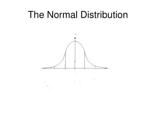
Importance • Many variables are distributed approximately as the bell-shaped normal curve • The mathematics of the normal curve are well known and relatively simple. • Many statistical procedures assume that the scores came from a normally distributed population.
Distributions of sums and means approach normality as sample size increases. • Many other probability distributions are closely related to the normal curve.
Using the Normal Curve • From its PDF (probability density function) we use integral calculus to find the probability that a randomly selected score would fall between value a and value b. • This is equivalent to finding what proportion of the total area under the curve falls between a and b.
The PDF • F(Y) is the probability density, aka the height of the curve at value Y. • There are only two parameters, the mean and the variance. • Normal distributions differ from one another only with respect to their mean and variance.
Avoiding the Calculus • Use the normal curve table in our text. • Use SPSS or another stats package. • Use an Internet resource.
IQ = 85, PR = ? • z = (85 - 100)/15 = -1. • What percentage of scores in a normal distribution are less than minus 1? • Half of the scores are less than 0, so you know right off that the answer is less than 50%. • Go to the normal curve table.
Normal Curve Table • For each z score, there are three values • Proportion from score to mean • Proportion from score to closer tail • Proportion from score to more distant tail
Locate the |z| in the Table • 34.13% of the scores fall between the mean and minus one. • 84.13% are greater than minus one. • 15.87% are less than minus one
IQ =115, PR = ? • z = (115 – 100)/15 = 1. • We are above the mean so the answer must be greater than 50%. • The answer is 84.13% .
85 < IQ < 115 • What percentage of IQ scores fall between 85 (z = -1) and 115 (z = 1)? • 34.13% are between mean and -1. • 34.13% are between mean and 1. • 68.26% are between -1 and 1.
115 < IQ < 130 • What percentage of IQ scores fall between 115 (z = 1) and 130 (z = 2)? • 84.13% fall below 1. • 97.72% fall below 2. • 97.72 – 84.13 = 13.59%
The Lowest 10% • What score marks off the lowest 10% of IQ scores ? • z = 1.28 • IQ = 100 – 1.28(15) = 80.8
The Middle 50% • What scores mark off the middle 50% of IQ scores? • -.67 < z < .67; • 100 - .67(15) = 90 • 100 + .67(15) = 110

