Download
1 / 18
400 likes | 1.35k Views
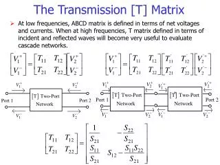
The Transmission [T] Matrix. At low frequencies, ABCD matrix is defined in terms of net voltages and currents. When at high frequencies, T matrix defined in terms of incident and reflected waves will become very useful to evaluate cascade networks. ‘. Equivalent Circuit for Two-Port Networks.

E N D
The Transmission [T] Matrix • At low frequencies, ABCD matrix is defined in terms of net voltages and currents. When at high frequencies, T matrix defined in terms of incident and reflected waves will become very useful to evaluate cascade networks. ‘
Equivalent Circuit for Two-Port Networks Acoax-to-microstrip transition and equivalent circuit representations. (a) Geometry of the transition. (b) Representation of the transition by a “black box.” (c) A possible equivalent circuit for the transition.
Equivalent circuits for some common microstrip discontinuities. (a) Open-ended. (b) Gap. (c) Change in width. (d) T-junction.
Equivalent circuits for a reciprocal two-port network. (a) T equivalent (b) equivalent
Example4.7: Find the network as equivalent T and model at 1GHz? Solution From Table 4-1 From Table 4-2
Equivalent T model From Table 4-2 Equivalent model
Example4.8: Find the equivalent model of microstrip-line inductor? Solution From Table 4-1 From Table 4-2
Example4.9: Find the equivalent T model of microstrip-line capacitor? Solution From Table 4-1 From Table 4-2
Problem3: Design a 6GHz attenuator ? (Hint: -20logS21=6 S21=0.501 ) • Problem4: Design a 6nH microstrip-line inductor on a 1.6mm thick FR4 substrate. The width of line is 0.25mm. Find the length (l ) and parasitic capacitance? • Problem5: Design a 2pF microstrip-line capacitor on a 1.6mm thick FR4 substrate. The width of line is 5mm. Find the length (l ) and parasitic inductance?
Chapter 5 Impedance Matching and Tuning
Why need Impedance Matching • Maximum power is delivered and power loss is minimum. • Impedance matching sensitive receiver components improves the signal-to-noise ratio of the system. • Impedance matching in a power distribution network will reduce amplitude and phase errors. • Basic Idea The matching network is ideally lossless and is placed between a load and a transmission line, to avoid unnecessary loss of power, and is usually designed so that the impedance seen looking into the matching network is Z0. ( Multiple reflections will exist between the matching network and the load) • The matching procedure is also referred to as “tuning”.
Design Considerations of Matching Network • As long as the load impedance has non-zero real part (i.e. Lossy term), a matching network can always be found. • Factors for selecting a matching network: 1) Complexity: a simpler matching network is more preferable because it is cheaper, more reliable, and less lossy. 2) Bandwidth: any type of matching network can ideally give a perfect match at a single frequency. However, some complicated design can provide matching over a range of frequencies. 3) Implementation: one type of matching network may be preferable compared to other methods. 4) Adjustability: adjustment may be required to match a variable load impedance.
Lumped Elements Matching • L-Shape (Two-Element) Matching • Case 1: ZL inside the 1+jx circle (RL>Z0) • Use impedance identity method
Example5.1: Design an L-section matching network to match a series RC load with an impedance ZL= 200-j100, to a 100 line, at a frequency of 500 MHz? Solution ( Use Smith chart) 1. Because the normalized load impedance ZL= 2-j1 inside the 1+jx circle, so case 1 network is select. 2. jB close to ZL, so ZL YL. 3. Move YL to 1+jx admittance circle, jB=j 0.3, where YL 0.4+j 0.5. 4. Then YLZL, ZL 1-j 1.2. So jX=j 1.2. 5. Impedance identity method derives jB=j 0.29 and jX=j 1.22. 6. Solution 2 uses jB=-j 0.7, where YL 0.4-j 0.5. 7. Then YLZL, ZL 1+j 1.2. So jX=-j 1.2. 8. Impedance identity method derives jB=-j 0.69 and jX=-j 1.22.