Download

1 / 14
140 likes | 280 Views
AEB 6184 – Concavity, Capital, and Panel Simulation. Elluminate – 7. Concavity. Among the conditions for the production function are positive marginal product and concavity (positive derivatives and negative definite or negative semi-definite hessian matrix)

E N D
AEB 6184 – Concavity, Capital, and Panel Simulation Elluminate – 7
Concavity • Among the conditions for the production function are positive marginal product and concavity (positive derivatives and negative definite or negative semi-definite hessian matrix) • As a starting point, I generate a sample of 150 observations using a quadratic production function.
Eigenvalues • The idea is to resample the dataset, keeping the observations which are concave. • The alternative is to directly impose the constraint that the eigenvalues are less than zero.
Production Function and the Theory of Capital • The student of economic theory has been taught to write where L is the quantity of labor, C is a quantity of capital, and O is the rate of output of commodities. • He is instructed to assume all workers alike, and to measure L in man-hours of labour; • He is told something about the index-number problem involved in choosing a unit of output; and • Then is hurried on to the next question, in hope that he will forget to ask in what units Cis measured. • Before ever he does ask, he has become a professor, and so sloppy habits of thought are handed on from one generation to another.
The question is certainly not an easy one to answer. • Capital in existence at any moment may be treated simply as “part of the environment in which labor works.” (Keynes – General Theory). • We then have a production function in terms of labour alone. • This is the right procedure for the short period within which supply of concrete capital goods does not alter, but outside the short period it is a very weak line to take, for it means that we cannot distinguish a change in the stock of capital (which can be made over the long run by accumulation) from a change in the weather (an act of God).
When we know the future expected rate of output associated with a certain capital good, and expect future prices and costs, then, if we are given a rate of interest, we can value the capital good as a discounted stream of future profit which it will earn. • But to do so, we have to begin by taking the rate of interest as given, whereas the main purpose of the production function is to show how wages and the rate of interest (regarded as the wages of capital) are determined.
Development of Panel Data • The idea or transition is that the amount of capital stock may determine individual components about the production function. • For example, assume that we have three inputs. • The first two are variable inputs (labor and materials). • The third is capital. • Taking a second-order Taylor series expansion
Next, allow the first two inputs to be variable while holding the third input fixed
Playing just a little fast and loose with the notation, we collapse the point of approximation into the constant of the quadratic function and then allow differences in the level of capital as a shift variable
Joan Robinson’s Point – Capital Levels could affect the marginal physical product of the other inputs
Changes in Isoquants • Selection problem by farm typology?
Rejoinder on Simulation of the firm under panel data (fixing the capital input).