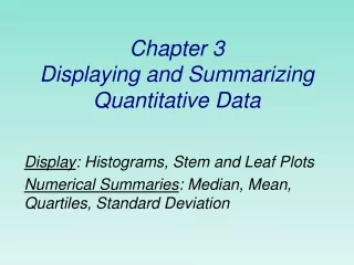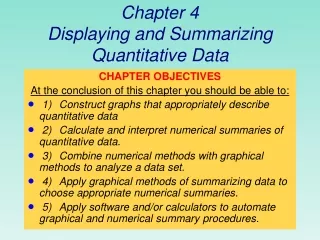
CHAPTER 4 Displaying and Summarizing Quantitative Data
CHAPTER 4 Displaying and Summarizing Quantitative Data. Slice up the entire span of values in piles called bins (or classes) Then count the number of values that fall in each bin The bins and the counts in each bin give the distribution of the quantitative variable. Histogram.

CHAPTER 4 Displaying and Summarizing Quantitative Data
E N D
Presentation Transcript
CHAPTER 4 Displaying and Summarizing Quantitative Data • Slice up the entire span of values in piles called bins (or classes) • Then count the number of values that fall in each bin • The bins and the counts in each bin give the distribution of the quantitative variable
Histogram • Display the counts in each bin in a histogram. • Like a bar chart, a histogram plots the bin counts as the heights of bars. • No spaces between bins. (different from a bar chart) • Relative frequency histogram displays percentage of cases in each bin instead of the count.
Stem and Leaf Display • Shows the distribution as well as the individual values. • Very Convenient: easy to make by hand. • Make a Steam and Leaf Display of the data set of exercise 40 (page 82)
Shape, Center, and Spread • How many Modes (“humps”)? • Histograms with • One peak Unimodal • Two peaks Bimodal • Three or more Multimodal • A histogram that doesn’t appear to have any mode and in which all the bars are approximately the same height is called Uniform • Exercise 7 Page 78
Symmetry • A distribution is symmetric if the two halves on either side of the center look approximately like mirror images of each other.
Skewed Distributions • Tails: The thinner ends of a distribution are called tails. If one tail stretches out farther than the other the histogram is said to be skewed to the side of the longer tail • Skew to the left Skew to the right
Outliers • Outliers are values that stand off away from the body of the distribution • Gaps in the distribution warn us that the data may not be homogeneous. They may come from different sources or contain more than one group. • (Example on page 52)
Center of the Distribution • For unimodal and symmetric distributions: • In the middle • For skewed and more than one mode is harder to find • (split in groups)
How Spread is the Distribution? • Just Checking page 56 • Comparing Distributions • Do men and women tend to get heart attacks at different ages?
Summarizing Distributions • Center • Midrange • Median: The middle value that divides the histogram into two equal areas • Order the values first • If n is odd the median is the middle value. Position (n+1)/2 • If n is even then take the average of the two middle values, that is the average of positions n/2 and n/2+1
Summarizing Distributions (cont.) • Spread • Range = Max – Min • Quartiles • Find the median, then find the median of each half. (Note: If n is odd include the median of the complete set to calculate the median of each half) • These are called the Lower quartile and Upper quartile and are denoted by Q1 and Q3 respectively.
The Interquartile Range • IQR = Q3 – Q1 • The lower and upper quartiles are also called the 25th and 75th percentiles • Q1 = 25th percentile • Median = 50th percentile • Q3 = 75th Percentile
Summarizing Distributions (cont.) • Summarizing Symmetric Distributions • If the shape of the distribution is symmetric, the mean (average) is a good alternative to summarize the distribution • Remember : Symmetric and no outliers • Mean:
Mean or Median • The mean is the point at which the histogram would balance. • Outliers will pull the mean in that direction. • For skewed data it’s better to report the median than the mean as a measure of center
What About Spread?The Standard Deviation • Standard Deviation: • It takes into account how far each value is from the mean • Appropriate only for symmetric data • Deviation: Distance from each data value to the mean • Variance • Standard Deviation
Shape, Center and Spread • Report always center and spread • Which measure for center and which measure for spread? • Skewed : Median and IQR • Symmetric: Mean and Standard Deviation • If there are outliers report the mean and standard deviations with and without the outliers. Median and IQR are not likely to be affected.
Chapter 5 Understanding and Comparing Distributions • After you have the five number summary you can create a display called a BoxPlot
Box Plots • Place the Median and quartiles over a line spanning the range of the data. (as shown in the board) • Locate the Upper and lower fences • Upper Fence = Q3 + 1.5 IQR • Lower Fence = Q1 – 1.5 IQR • Then draw the Whiskers (Most Extreme data value Found within the fences) • Display Outliers
Exercise • Comparing Groups (Page 93)
Time Plot • Displays data that changes over time • (What is wrong with the time plot on page 104?)