Transport Layer

1. Transport Layer Dr. Nawaporn Wisitpongphan Credit: Prof. Nick McKeown http://www.stanford.edu/~nickm

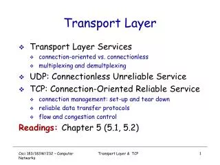
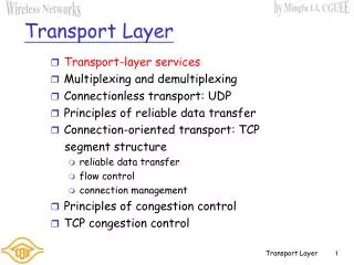
2. Outline • The Transport Layer • The UDP Protocol • The TCP Protocol • TCP Characteristics • TCP Connection setup • TCP Segments • TCP Sequence Numbers • TCP Sliding Window • Timeouts and Retransmission • Congestion Control and Avoidance

3. Application Layer Transport Layer O.S. O.S. Network Layer Link Layer D D D D D D H H H H H H Data Data Header Header Review of the transport layer Athena.MIT.edu Leland.Stanford.edu Nick Dave

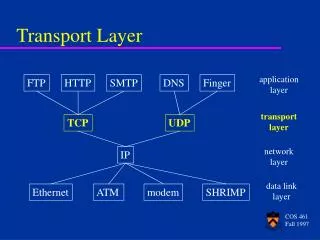
4. Layering: The OSI Model layer-to-layer communication Application Application 7 7 Presentation Presentation 6 6 Session Session 5 5 Peer-layer communication Transport Transport Router Router 4 4 Network Network Network Network 3 3 Link Link Link Link 2 2 Physical Physical Physical Physical 1 1

5. User Datagram Protocol (UDP) Characteristics • UDP is a connectionless datagram service. • There is no connection establishment: packets may show up at any time. • UDP is unreliable: • No acknowledgements to indicate delivery of data. • Checksums cover the header, and only optionally cover the data. • Contains no mechanism to detect missing or mis-sequenced packets. • No mechanism for automatic retransmission. • No mechanism for flow control, and so can over-run the receiver.

6. User-Datagram Protocol (UDP) A1 A2 B1 B2 App App App App OS UDP UDP uses port number to demultiplex packets IP

7. User-Datagram Protocol (UDP)Packet format SRC port DST port By default, only covers the header. checksum length DATA • Why do we have UDP? • It is used by applications that don’t need reliable delivery, or • Applications that have their own special needs, such as streaming of real-time audio/video.

8. TCP Characteristics • TCP is connection-oriented. • 3-way handshake used for connection setup. • TCP provides a stream-of-bytes service. • TCP is reliable: • Acknowledgements indicate delivery of data. • Checksums are used to detect corrupted data. • Sequence numbers detect missing, or mis-sequenced data. • Corrupted data is retransmitted after a timeout. • Mis-sequenced data is re-sequenced. • (Window-based) Flow control prevents over-run of receiver. • TCP uses congestion control to share network capacity among users.

9. HTTP and TCP

10. TCP is connection-oriented (Active) Client (Passive) Server (Active) Client (Passive) Server Syn Fin Syn + Ack (Data +) Ack Ack Fin Ack Connection Setup 3-way handshake Connection Close/Teardown 2 x 2-way handshake

11. The TCP Diagram (Active) Client (Passive) Server Syn Syn + Ack Which path does the Active Client or Passive Server follow? Ack

12. TCP Client

13. TCP Server

14. TCP supports a “stream of bytes” service • TCP accepts data as a constant stream from the applications • There are no record markers automatically inserted by TCP. • Example: • If the application on one end writes 10 bytes, followed by a write of 20 bytes, followed by a write of 50 bytes, the application at the other end of the connection cannot tell what size the individual writes were. The other end may read the 80 bytes in four reads of 20 bytes at a time. • One end puts a stream of bytes into TCP and the same, identical stream of bytes appears at the other end Host A Byte 0 Byte 1 Byte 2 Byte 3 Byte 80 Byte 0 Byte 1 Byte 2 Byte 3 Byte 80 Host B

15. …which is emulated using TCP “segments” Host A Byte 0 Byte 1 Byte 2 Byte 3 Byte 80 • Segment sent when: • Segment full (MSS bytes), • Not full, but times out, or • “Pushed” by application. TCP Data TCP Data Host B Byte 0 Byte 1 Byte 2 Byte 3 Byte 80

16. The TCP Segment Format IP Data IP Hdr TCP Data TCP Hdr 0 15 31 Src port Dst port Sequence # Src/dst port numbers and IP addresses uniquely identify socket Ack Sequence # TCP Header and Data + IP Addresses Flags Window Size RSVD 6 HLEN 4 SYN PSH URG RST FIN ACK Checksum Urgent Pointer (TCP Options) TCP Data

17. Sequence Numbers How does ISN get chosen? Host A ISN (initial sequence number) Sequence number = 1st byte TCP HDR TCP Data Ack sequence number = next expected byte TCP HDR TCP Data Host B

18. Initial Sequence Numbers (Active) Client (Passive) Server Sequence number = 32 bits What if a message has more than 232bytes? Syn +ISNA Syn + Ack +ISNB Sequence Number wrap-around Ack Connection Setup 3-way handshake Solution : Timestamp Option : Sender places timestamp in every segment : Receiver copies timestamp in the ACK it sends for a segment

19. TCP Sliding Window • How much data can a TCP sender have outstanding in the network? • How much data should TCP retransmit when an error occurs? Just selectively repeat the missing data? • How does the TCP sender avoid over-running the receiver’s buffers?

20. TCP Sliding Window Window Size Data ACK’d Outstanding Un-ack’d data Data OK to send Data not OK to send yet • Window is meaningful to the sender. • Current window size is “advertised” by receiver • (usually 4k – 8k Bytes when connection set-up).

21. Round-trip time Window Size Window Size ??? ACK (2) RTT = Window size TCP Sliding Window Round-trip time Window Size Host A Host B ACK ACK (1) RTT > Window size

22. TCP: Retransmission and Timeouts Round-trip time (RTT) Retransmission TimeOut (RTO) Guard Band Host A Estimated RTT Data1 Data2 ACK ACK Host B • TCP uses an adaptive retransmission timeout value: • Congestion • Changes in Routing RTT changes frequently

23. TCP: Retransmission and Timeouts • Picking the RTO is important: • Pick a values that’s too big and it will wait too long to retransmit a packet, • Pick a value too small, and it will unnecessarily retransmit packets. • The original algorithm for picking RTO: • EstimatedRTTk=  EstimatedRTTk-1 + (1 - ) SampleRTT • RTO = 2 * EstimatedRTT • Characteristics of the original algorithm: • Variance is assumed to be fixed. • But in practice, variance increases as congestion increases. Determined empirically

24. Average Queueing Delay Variance grows rapidly with load Load (Amount of traffic arriving to router) TCP: Retransmission and Timeouts • Router queues grow when there is more traffic, until they become unstable. • As load grows, variance of delay grows rapidly. • There will be some (unknown) distribution of RTTs. • We are trying to estimate an RTO to minimize the probability of a false timeout. Probability variance RTT mean

25. TCP: Retransmission and Timeouts • Newer Algorithm includes estimate of variance in RTT: • Difference = SampleRTT - EstimatedRTT • EstimatedRTTk = EstimatedRTTk-1 + (*Difference) • Deviation = Deviation + *( |Difference| - Deviation ) • RTO =  * EstimatedRTT +  * Deviation •   1 •   4 Same as before

26. TCP: Retransmission and TimeoutsKarn’s Algorithm Host A Host B Host A Host B Retransmission Retransmission Wrong RTT Sample Wrong RTT Sample Problem: How can we estimate RTT when packets are retransmitted? Solution: On retransmission, don’t update estimated RTT (and double RTO).

27. Congestion Control: Main points • Congestion is inevitable • Congestion happens at different scales – from two individual packets colliding to too many users • TCP Senders can detect congestion and reduce their sending rate by reducing the window size • TCP modifies the rate according to “Additive Increase, Multiplicative Decrease (AIMD)”. • To probe and find the initial rate, TCP uses a restart mechanism called “slow start”. • Routers slow down TCP senders by buffering packets and thus increasing delay

28. Congestion A1(t) 10Mb/s H1 R1 D(t) 1.5Mb/s H3 A2(t) 100Mb/s H2 A1(t) D(t) A2(t) X(t) A2(t) Cumulative bytes A1(t) X(t) D(t) t

29. Time Scales of Congestion Too many users using a link during a peak hour 7:00 8:00 9:00 TCP flows filling up allavailable bandwidth 1s 2s 3s Two packets collidingat a router 100µs 200µs 300µs

30. Dealing with CongestionExample: two flows arriving at a router A1(t) ? R1 A2(t)

31. Congestion is unavoidableArguably it’s good! • We use packet switching because it makes efficient use of the links. Therefore, buffers in the routers are frequently occupied. • If buffers are always empty, delay is low, but our usage of the network is low. • If buffers are always occupied, delay is high, but we are using the network more efficiently. • So how much congestion is too much?

32. Load, delay and power Typical behavior of queueing systems with random arrivals: A simple metric of how well the network is performing: Burstiness tends to move asymptote to the left Power Average Packet delay Load Load “optimal load”

33. Options for Congestion Control • Implemented by host versus network • Reservation-based, versus feedback-based • Window-based versus rate-based.

34. TCP Congestion Control • TCP implements host-based, feedback-based, window-based congestion control. • TCP sources attempts to determine how much capacity is available • TCP sends packets, then reacts to observable events (loss).

35. TCP Congestion Control • TCP sources change the sending rate by modifying the window size: Window = min{Advertized window, Congestion Window} • In other words, send at the rate of the slowest component: network or receiver. • “cwnd” follows additive increase/multiplicative decrease • On receipt of Ack: cwnd += 1 • On packet loss (timeout): cwnd *= 0.5 Receiver Transmitter (“cwnd”)

36. Additive Increase/ Multiplicative Decrease Src D D A A D D D A A A D A Dest Additive Increase: Every time the source successfully sends a cwnd’s worth of packets (each pkt sent out during the last RTT has been ACKed)  add the equivalent of 1 pkt to the cwnd Increment = MSS×(MSS/CWND) ; CWND≥MSS CWND +=Increment

37. Leads to the TCP “sawtooth” Window Timeouts Could take a long time to get started! halved t Multiplicative Decrease: For each timeout, the source set CWND to half of its previous value. • CWND is large • all the packets dropped will be retransmitted  congestion gets worse • Need to get out of this state quickly

38. “Slow Start” • Designed to find the fair-share rate quickly at startup. • How Does it work? • Increase cwnd exponentially for each ACK received, until it reaches SSthreshold. • If cwnd < SSthreshold {Do Slow Start}, else {Do Congestion Avoidance} • Initial SSThreshold = large value. After the pkt lost, SSThreshold = cwnd/2 • Congestion Avoidance Increase cwnd linearly 1 2 4 8 Src D D D A A D D D D A A A A A Dest

39. Slow Start Why is it called slow-start? Because TCP originally had no congestion control mechanism. The source would just start by sending a whole advertised window’s worth of data.

40. Fast Retransmit and Fast Recovery? Homework!!

41. TCP Sending Rate • What is the sending rate of TCP? • Acknowledgement for sent packet is received after one RTT • Amount of data sent until ACK is received is the current window size W • Therefore sending rate is R = W/RTT • Is the TCP sending rate saw tooth shaped as well?

42. TCP and buffers

43. TCP and Buffers • For TCP with a single flow over a network link with enough buffers, RTTand Ware proportional to each other • Therefore the sending rate R = W/RTTis constant (and not a sawtooth) • But experiments and theory suggest that with many flows: Where: p is the drop probability. • TCP rate can be controlled in two ways: • Buffering packets and increasing the RTT • Dropping packets to decrease TCP’s window size

44. Congestion control in the Internet • Maximum window sizes of most TCP implementations by default are very small • Windows XP: 12 packets • Linux/Mac: 40 packets • Often the buffer of a link is larger than the maximum window size of TCP • A typical DSL line has 200 packets worth of buffer • For a TCP session, the maximum number of packets outstanding is 40 • The buffer can never fill up • The router will never drop a packet

45. Average Packet delay Load Congestion Avoidance • TCP reacts to congestion after it takes place. The data rate changes rapidly and the system is barely stable (or is even unstable). • Can we predict when congestion is about to happen and avoid it? E.g. by detecting the knee of the curve.

46. Congestion Avoidance Schemes • Router-based Congestion Avoidance: • DECbit: • Routers explicitly notify sources about congestion. • Random Early Detection (RED): • Routers implicitly notify sources by dropping packets. • RED drops packets at random, and as a function of the level of congestion. • Host-based Congestion Avoidance • Source monitors changes in RTT to detect onset of congestion.

47. DECbit • Each packet has a “Congestion Notification” bit called the DECbit in its header. • If any router on the path is congested, it sets the DECbit. • Set if average queue length >= 1 packet, averaged since the start of the previous busy cycle. • To notify the source, the destination copies DECbit into ACK packets. • Source adjusts rate to avoid congestion. • Counts fraction of DECbits set in each window. • If <50% set, increase rate additively. • If >=50% set, decrease rate multiplicatively. Queue Lengthat router Time Averaging period

48. Random Early Detection (RED) • RED is based on DECbit, and was designed to work well with TCP. • RED implicitly notifies sender by dropping packets. • Drop probability is increased as the average queue length increases. • (Geometric) moving average of the queue length is used so as to detect long term congestion, yet allow short term bursts to arrive.

49. RED Drop Probabilities D(t) A(t) 1 maxP AvgLen minTh maxTh

50. Properties of RED • Drops packets before queue is full, in the hope of reducing the rates of some flows. • Drops packet for each flow roughly in proportion to its rate. • Drops are spaced out in time. • Because it uses average queue length, RED is tolerant of bursts. • Random drops hopefully desynchronize TCP sources.