Download
1 / 67
670 likes | 848 Views
CS520 Advanced Analysis of Algorithms and Complexity. Dr. Ben Choi Ph.D. in EE (Computer Engineering), The Ohio State University System Performance Engineer, Lucent Technologies - Bell Labs Innovations Pilot, FAA certified pilot for airplanes and helicopters BenChoi.info.

E N D
CS520 Advanced Analysis of Algorithms and Complexity Dr. Ben Choi Ph.D. in EE (Computer Engineering), The Ohio State University System Performance Engineer, Lucent Technologies - Bell Labs Innovations Pilot, FAA certified pilot for airplanes and helicopters BenChoi.info
What is a Computer Algorithm? • A computer algorithm is • a detailed step-by-step method for • solving a problem • by using a computer.
Problem-Solving (Science and Engineering) • Analysis • How does it work? • Breaking a system down to known components • How the components relate to each other • Breaking a process down to known functions • Synthesis • Building tools and toys! • What components are needed • How the components should be put together • Composing functions to form a process
Problem Solving Using Computers • Problem: • Strategy: • Algorithm: • Input: • Output: • Step: • Analysis: • Correctness: • Time & Space: • Optimality: • Implementation: • Verification:
Example: Search in an unordered array • Problem: • Let E be an array containing n entries, E[0], …, E[n-1], in no particular order. • Find an index of a specified key K, if K is in the array; • return –1 as the answer if K is not in the array. • Strategy: • Compare K to each entry in turn until a match is found or the array is exhausted. • If K is not in the array, the algorithm returns –1 as its answer.
Example: Sequential Search, Unordered • Algorithm (and data structure) • Input: E, n, K, where E is an array with n entries (indexed 0, …, n-1), and K is the item sought. For simplicity, we assume that K and the entries of E are integers, as is n. • Output: Returns ans, the location of K in E (-1 if K is not found.)
Algorithm: Step (Specification) • int seqSearch(int[] E, int n, int K) • 1. int ans, index; • 2. ans = -1; // Assume failure. • 3. for (index = 0; index < n; index++) • 4. if (K == E[index]) • 5. ans = index; // Success! • 6. break; // Done! • 7. return ans;
Analysis of the Algorithm • How shall we measure the amount of work done by an algorithm? • Basic Operation: • Comparison of x with an array entry • Worst-Case Analysis: • Let W(n) be a function. W(n) is the maximum number of basic operations performed by the algorithm on any input size n. • For our example, clearly W(n) = n. • The worst cases occur when K appears only in the last position in the array and when K is not in the array at all.
More Analysis of the Algorithm • Average-Behavior Analysis: • Let q be the probability that K is in the array • A(n) = n(1 – ½ q) + ½ q • Optimality: • The Best possible solution? • Searching an Ordered Array • Using Binary Search • W(n) = Ceiling[lg(n+1)] • The Binary Search algorithm is optimal. • Correctness: (Proving Correctness of Procedures s3.5)
What is CS 520? • Class Syllabus
Algorithm Language (Specifying the Steps) • Java as an algorithm language • Syntax similar to C++ • Some steps within an algorithm may be specified in pseduocode (English phrases) • Focus on the strategy and techniques of an algorithm, not on detail implementation
Analysis Tool: Mathematics: Set • A set is a collection of distinct elements. • The elements are of the same “type”, common properties. • “element e is a member of set S” is denoted as e S • Read “e is in S” • A particular set is defined by listing or describing its elements between a pair of curly braces:S1 = {a, b, c}, S2 = {x | x is an integer power of 2}read “the set of all elements x such that x is …” • S3 = {} = , has not elements, called empty set • A set has no inherent order.
Subset, Superset; Intersection, Union • If all elements of one set, S1 • are also in another set, S2, • Then S1 is said to be a subset of S2, S1 S2 • and S2 is said to be a superset of S1, S2 S1. • Empty set is a subset of every set, S • Intersection • S T = {x | x S and x T} • Union • S T = {x | x S or x T}
Cardinality • Cardinality • A set, S, is finite if there is an integer n such that the elements of S can be placed in a one-to-one correspondence with {1, 2, 3, …, n} • in this case we write |S| = n • How many distinct subsets does a finite set on n elements have? There are 2n subsets. • How many distinct subsets of cardinality k does a finite set of n elements have? There are C(n, k) = n!/((n-k)!k!), “n choose k”
Sequence • A group of elements in a specified order is called a sequence. • A sequence can have repeated elements. • Sequences are defined by listing or describing their elements in order, enclosed in parentheses. • e.g. S1 = (a, b, c), S2 = (b, c, a), S3 = (a, a, b, c) • A sequence is finite if there is an integer n such that the elements of the sequence can be placed in a one-to-one correspondence with (1, 2, 3, …, n). • If all the elements of a finite sequence are distinct, that sequence is said to be a permutation of the finite set consisting of the same elements. • One set of n elements has n! distinct permutations.
Tuples and Cross Product • A tuple is a finite sequence. • Ordered pair (x, y), triple (x, y, z), quadruple, and quintuple • A k-tuple is a tuple of k elements. • The cross product of two sets, say S and T, isS T = {(x, y) | x S, y T} • | S T | = |S| |T| • It often happens that S and T are the same set, e.g. N Nwhere N denotes the set of natural numbers, {0,1,2,…}
Relations and Functions • A relation is some subset of a (possibly iterated) cross product. • A binary relation is some subset of a cross product,e.g. R S T • e.g. “less than” relation can be defined as {(x, y) | x N, y N, x < y} • Important properties of relations; let R S S • reflexive: for all x S, (x, x) R. • symmetric: if (x, y) R, then (y, x) R. • antisymmetric: if (x, y) R, then (y, x) R • transitive: if (x,y) R and (y, z) R, then (x, z) R. • A relation that is reflexive, symmetric, and transitive is called an equivalence relation, partition the underlying set S into equivalence classes [x] = {y S | x R y}, x S • A function is a relation in which no element of S (of S x T) is repeated with the relation. (informal def.)
Analysis Tool: Logic • Logic is a system for formalizing natural language statements so that we can reason more accurately. • The simplest statements are called atomic formulas. • More complex statements can be build up through the use of logical connectives: “and”, “or”, “not”, “implies” A B “A implies B” “if A then B” • A B is logically equivalent to A B • (A B) is logically equivalent to A B • (A B) is logically equivalent to A B
Quantifiers: all, some • “for all x” x P(x) is true iff P(x) is true for all x • universal quantifier (universe of discourse) • “there exist x” x P(x) is true iff P(x) is true for some value of x • existential quantifier • x A(x) is logically equivalent to x(A(x)) • x A(x) is logically equivalent to x(A(x)) • x (A(x) B(x)) “For all x such that if A(x) holds then B(x) holds”
Prove: by counterexample, Contraposition, Contradiction • Counterexampleto prove x (A(x) B(x)) is false, we show some object x for which A(x) is true and B(x) is false. • (x (A(x) B(x))) x (A(x) B(x)) • Contrapositionto prove A B, we show ( B) ( A) • Contradictionto prove A B, we assume B and then prove B. • A B (A B) B • A B (A B) is false • Assuming (A B) is true, and discover a contradiction (such as A A), then conclude (A B) is false, and so A B.
Prove: by Contradiction, e.g. • Prove [B (B C)] C • by contradiction • Proof: • Assume C • C [B (B C)] • C [B ( B C)] • C [(B B) (B C)] • C [(B C)] • C C B • False, Contradiction • C
Rules of Inference • A rule of inference is a general pattern that allows us to draw some new conclusion from a set of given statements. • If we know {…} then we can conclude {…} • If {B and (B C)} then {C} • modus ponens • If {A B and B C} then {A C} • syllogism • If {B C and B C} then {C} • rule of cases
Two-valued Boolean (algebra) logic • 1. There exists two elements in B, i.e. B={0,1} • there are two binary operations + “or, ”, · “and, ” • 2. Closure: if x, y B and z = x + y then z B • if x, y B and z = x · y then z B • 3. Identity element: for + designated by 0: x + 0 = x • for · designated by 1: x · 1 = x • 4. Commutative: x + y = y + x • x · y = y · x • 5. Distributive: x · (y + z) = (x · y) + (x · z) • x + (y · z) = (x + y) · (x + z) • 6. Complement: for every element x B, there exits an element x’ B • x + x’ = 1, x · x’ = 0
True Table and Tautologically Implies e.g. • Show [B (B C)] C is a tautology: • B C (B C) [B (B C)] [B (B C)] C • 0 0 1 0 1 • 0 1 1 0 1 • 1 0 0 0 1 • 1 1 1 1 1 • For every assignment for B and C, • the statement is True
Prove: by Rule of inferences • Prove [B (B C)] C • Proof: • [B (B C)] C • [B (B C)] C • [B ( B C)] C • [(B B) (B C)] C • [(B C)] C • B C C • True (tautology) • Direct Proof: • [B (B C)] [B C] C
Analysis Tool: Probability • Elementary events (outcomes) • Suppose that in a given situation an event, or experiment, may have any one, and only one, of k outcomes, s1, s2, …, sk. (mutually exclusive) • Universe The set of all elementary events is called the universe and is denoted U = {s1, s2, …, sk}. • Probability of si • associate a real number Pr(si), such that • 0 Pr(si) 1 for 1 i k; • Pr(s1) + Pr(s2) + … + Pr(sk) = 1
Event • Let S U. Then S is called an event, and • Pr(S) = si S Pr(si) • Sure event U = {s1, s2, …, sk}, Pr(U) = 1 • Impossible event, ,Pr() = 0 • Complement event “not S” U – S, Pr(not S) = 1 – Pr(S)
Conditional Probability • The conditional probability of an event S given an event T is defined as • Pr(S | T) = Pr(S and T) / Pr(T) = si ST Pr(si) / sj T Pr(sj) • Independent • Given two events S and T, if • Pr(S and T) = Pr(S)Pr(T) • then S and T are stochastically independent, or simply independent.
Random variable and their Expected value • A random variable is a real valued variable that depends on which elementary event has occurred • it is a function defined for elementary events. • e.g. f(e) = the number of inversions in the permutation of {A, B, C}; assume all input permutations are equally likely. • Expectation • Let f(e) be a random variable defined on a set of elementary events e U. The expectation of f, denoted as E(f), is defined as • E(f) = e U f(e)Pr(e) • This is often called the average values of f. • Expectations are often easier to manipulate then the random variables themselves.
Conditional expectation and Laws of expectations • The conditional expectation of f given an event S, denoted as E (f | S), is defined as • E(f | S) = e S f(e)Pr(e | S) • Law of expectations • For random variables f(e) and g(e) defined on a set of elementary events e U, and any event S: • E(f + g) = E(f) + E(g) • E(f) = Pr(S)E(f | S) + Pr(not S) E(f | not S)
Analysis Tool: Algebra • Manipulating Inequalities • Transitivity: If ((A B) and (B C) Then (A C) • Addition: If ((A B) and (C D) Then (A+C B+D) • Positive Scaling: If ((A B) and (> 0) Then ( A B) • Floor and Ceiling Functions • Floor[x] is the largest integer less than or equal to x. • Ceiling[x] is the smallest integer greater than or equal to x.
Logarithms • For b>1 and x>0, logbx (read “log to the base b of x”) is that real number L such that bL = x • logbx is the power to which b must be raised to get x. • Log properties: def: lg x = log2 x; ln x = loge x • Let x and y be arbitrary positive real numbers, let a, b any real number, and let b>1 and c>1 be real numbers. • logb is a strictly increasing function, if x > y then logb x > logb y • logb is a one-to-one function, if logb x = logb y then x = y • logb 1 = 0; logb b = 1; logb xa = a logb x • logb(xy) = logb x + logb y • xlog y = ylog x • change base: logcx = (logb x)/(logb c)
Series • A series is the sum of a sequence. • Arithmetic series • The sum of consecutive integers • Polynomial Series • The sum of squares • The general case is • Power of 2 • Arithmetic- • Geometric Series
Summations Using Integration • A function f(x) is said to be monotonic, or nondecreasing, if x y always implies that f(x) f(y). • A function f(x) is antimonotonic, or nonincreasing, if –f(x) is monotonic. • If f(x) is nondecreasing then • If f(x) is nonincreasing then
g Classifying functions by theirAsymptotic Growth Rates • asymptotic growth rate, asymptotic order, or order of functions • Comparing and classifying functions that ignores constant factors and small inputs. • The Sets big oh O(g), big theta (g), big omega (g) (g): functions that grow at least as fast as g (g): functions that grow at the same rate as g O(g): functions that grow no faster than g
The Sets O(g), (g), (g) • Let g and f be a functions from the nonnegative integers into the positive real numbers • For some real constant c > 0 and some nonnegative integer constant n0 • O(g) is the set of functions f, such that • f(n) c g(n) for all n n0 • (g) is the set of functions f, such that • f(n) c g(n) for all n n0 • (g) = O(g) (g) • asymptotic order of g • f (g) read as “f is asymptotic order g” or “f is order g”
Comparing asymptotic growth rates • Comparing f(n) and g(n) as n approaches infinity, • IF • < , including the case in which the limit is 0 then f O(g) • > 0, including the case in which the limit is then f (g) • = c and 0 < c < then f (g) • = 0 then f o(g) //read as “little oh of g” • = then f (g) //read as “little omega of g”
Properties of O(g), (g), (g) • Transitive: If f O(g) and g O(h), then f O(h)O is transitive. Also , , o, are transitive. • Reflexive: f (f) • Symmetric: If f (g), then g (f) • defines an equivalence relation on the functions. • Each set (f) is an equivalence class (complexity class). • f O(g) g (f) • O(f + g) = O(max(f, g)) similar equations hold for and
Classification of functions, e.g. • O(1) denotes the set of functions bounded by a constant (for large n) • f (n), f is linear • f (n2), f is quadratic; f (n3), f is cubic • lg n o(n) for any > 0, including factional powers • nk o(cn) for any k > 0 and any c > 1 • powers of n grow more slowly than any exponential function cn
Analyzing Algorithms and Problems • We analyze algorithms with the intention ofimproving them, if possible, and for choosing among several available for a problem. • Correctness • Amount of work done, and space used • Optimality, Simplicity
Correctness can be proved! • An algorithm consists of sequences of steps (operations, instructions, statements) for transforminginputs (preconditions) to outputs (postconditions) • Proving • if the preconditions are satisfied, • then the postconditions will be true, • when the algorithm terminates.
Amount of work done • We want a measure of work that tells us something about the efficiency of the method used by the algorithm • independent of computer, programming language, programmer, and other implementation details. • Usually depending on the size of the input • Counting passes through loops • Basic Operation • Identify a particular operation fundamental to the problem • the total number of operations performed is roughly proportional to the number of basic operations • Identifying the properties of the inputs that affect the behavior of the algorithm
Worst-case complexity • Let Dn be the set of inputs of size n for the problem under consideration, and let I be an element of Dn. • Let t(I) be the number of basic operations performed by the algorithm on input I. • We define the function W by • W(n) = max{t(I) | I Dn} • called the worst-case complexity of the algorithm. • W(n) is the maximum number of basic operations performed by the algorithm on any input of size n. • The input, I, for which an algorithm behaves worstdepends on the particular algorithm.
Average Complexity • Let Pr(I) be the probability that input I occurs. • Then the average behavior of the algorithm is defined as • A(n) = I Dn Pr(I) t(I). • We determine t(I) by analyzing the algorithm, • but Pr(I) cannot be computed analytically. • A(n) = Pr(succ)Asucc(n) + Pr(fail)Afail(n) • An element I in Dn may be thought as a set or equivalence class that affect the behavior of the algorithm. (see following e.g. n+1 cases)
e.g. Search in an unordered array • int seqSearch(int[] E, int n, int K) • 1. int ans, index; • 2. ans = -1; // Assume failure. • 3. for (index = 0; index < n; index++) • 4. if (K == E[index]) • 5. ans = index; // Success! • 6. break; // Done! • 7. return ans;
Average-Behavior Analysis e.g. • A(n) = Pr(succ)Asucc(n) + Pr(fail)Afail(n) • There are total of n+1 cases of I in Dn • Let K is in the array as “succ” cases that have n cases. • Assuming K is equally likely found in any of the n location, i.e. Pr(Ii | succ) = 1/n • for 0 <= i < n, t(Ii) = i + 1 • Asucc(n) = i=0n-1Pr(Ii | succ) t(Ii) • = i=0n-1(1/n) (i+1) = (1/n)[n(n+1)/2] = (n+1)/2 • Let K is not in the array as the “fail” case that has 1 cases, Pr(I | fail) = 1 • Then Afail(n) = Pr(I | fail) t(I) = 1 n • Let q be the probability for the succ cases • q [(n+1)/2] + (1-q) n
Space Usage • If memory cells used by the algorithms depends on the particular input, • then worst-case and average-case analysis can be done. • Time and Space Tradeoff.
Optimality “the best possible” • Each problem has inherent complexity • There is some minimum amount of work required to solve it. • To analyze the complexity of a problem, • we choose a class of algorithms, based on which • prove theorems that establish a lower bound on the number of operations needed to solve the problem. • Lower bound (for the worst case)
Show whether an algorithm is optimal? • Analyze the algorithm, call it A, and found the Worst-case complexity WA(n), for input of size n. • Prove a theorem starting that, • for any algorithm in the same class of A • for any input of size n, there is some input for which the algorithm must perform • at least W[A](n) (lower bound in the worst-case) • If WA(n) == W[A](n) • then the algorithm A is optimal • else there may be a better algorithm • OR there may be a better lower bound.
Optimality e.g. • Problem • Fining the largest entry in an (unsorted) array of n numbers • Algorithm A • int findMax(int[] E, int n) • 1. int max; • 2. max = E[0]; // Assume the first is max. • 3. for (index = 1; index < n; index++) • 4. if (max < E[index]) • 5. max = E[index]; • 6. return max;