Download
1 / 26
260 likes | 279 Views
The ATLAS tracking and vertexing detector. Introduction ATLAS & LHC Tracking and Vertexing in ATLAS Conclusions. one hit pattern (image) = trails left by ionizing particles = 1event Information concentrated in some special events (to be hunted for)

E N D
The ATLAS tracking and vertexing detector • Introduction • ATLAS & LHC • Tracking and Vertexing in ATLAS • Conclusions Leonardo Rossi – CERN&INFN-Genoa
one hit pattern (image) = trails left by ionizing particles = 1event Information concentrated in some special events (to be hunted for) Interesting events must be selected (trigger + analysis) one image is made of many events (e.g. many X-ray conversions) Information distributed in all events Summing-up enough events give the required image quality Particle physics and imaging Leonardo Rossi – CERN&INFN-Genoa
Higher energies & luminosities s(nb) • Particle physics trends higher energies • explore smaller details of the matter (l=h/p) • have access to higher masses (E=mc2) but also higher interaction rate (= machine luminosity) • The events of interest (higher mass) are rare • …and “buried” m¥, hot universe, t0 Leonardo Rossi – CERN&INFN-Genoa
The most economic way of getting high-E and L is p-p collisions • protons are complex objects: • Only hard collisions are useful • A lot of background collisions • Effective energy available: =Ö X1 X2 E2 • wide band energy beams • useful to explore new E-window • few energetic collisions • need to select them X2 X1 Leonardo Rossi – CERN&INFN-Genoa
Tracking at LHC • Large Hadron Collider in operation next year • Circumf ~27km, E=14 TeV, L=1034 cm-2s-1,40MHz x-ing • 1 GHz interaction rate, 103 particles each 25 ns. • Tracking detectors must then be: • Fast (40MHz), Rad-Hard (10-100kGy), high granularity & good pattern recognition capabilities (103 tks/25 ns). • Environment is hostile, why measuring tracks? • To measure momenta (dynamics, invariant masses) • To measure vertices • Primary improve on p and E measurements • Secondary tag ps living particles (b,t) markers of events with significant physics content • To help identifying photons Leonardo Rossi – CERN&INFN-Genoa
ATLAS tracking • General guidelines of ATLAS tracker design • Outer shell R[56-108 cm] continuous tracking (~30 hits per track) with closely packed gaseous detectors (TransitionRadiationTracker) • Inner shell R[5-60 cm] discrete tracking with higher precision silicon detectors • Outside microstrip detectors (SiliConTracker) • Inside pixel detectors (Pixel) (higher granularity and radiation hardness) • Let’s flash trough ATLAS and then concentrate on tracking and vertexing Leonardo Rossi – CERN&INFN-Genoa
Magnet system ( 2Tesla) The ATLAS Detector Inner Detector = Tracker Muon Spectrometer Calorimeter Leonardo Rossi – CERN&INFN-Genoa
The ATLAS Tracker Inside a 2T solenoidal B-field Barrel TRT End Cap TRT End Cap SCT ~2.2m Pixels ~5.5m Barrel SCT • Layout is split in 4 parts (installed separately): • Barrel (SCT+TRT): cylindrical geometry • 2 Forward Sections ( both SCT+TRT): disk geometry • Pixel (+ beam-pipe) (cylindrical + disk geometry) acceptance: -2.5<h<2.5 h=-ln tan(q/2) q=azimuth Leonardo Rossi – CERN&INFN-Genoa
The Tracking Detectors (inside out) Pixel: Barrel: 3 layers (R=5.1, 8.9, 12.3 cm). Endcap:2 x 3 disks of Silicon pixel detectors (Rin=9, Rout=15 cm) Building block: the module (1744 all equal, covering 1.7 m2, 46080 channels each (then 80 106 channels), 250 mm thick, pitch 50 x 400 mm) 130 cm 60.8 mm Top view Side view - sketch (not to scale) 0.2mm thick sensor 16.4 mm 16 front-end chips Leonardo Rossi – CERN&INFN-Genoa
Working principle: ionization in small volume (0.05 x 0.4 x 0.2 mm3) Si. All volumes contiguous (full surface sensitive). Electronics matrix matches sensor matrix connection out-of-plane (bump bonding) Advantages: small C (good S/N, fast), small I + can operate partially depleted (rad-hardness), excellent PR capability Drawbacks: cost/cm2, power density Leonardo Rossi – CERN&INFN-Genoa
Key ATLAS Pixel Results Efficiency after 500 kGy Time resolution vs charge signal e = 98.7±0.7% (0kGy99.9%) Plateau =9.7± 1.1 ns (0kGy14ns) Leonardo Rossi – CERN&INFN-Genoa
Space resolution 500 kGy 0 kGy =9.7 m =7.5 m only binary readout Leonardo Rossi – CERN&INFN-Genoa
SCT: Barrel: 4 cylinders (R~30 , 37, 44 and 51 cm) EndCap: 9 disks per side (Rin-min~27, Rout~56 cm) 9 disks 4 cylinders 12 cm Building block: the module (back-to-back single sided Si microstrip sensors 285 mm thick, 80 mm pitch). 2112(b)+1976(ec) modules covering 61 m2 with 6.2 106 channels. 40 mRad stereo Barrel module 6 cm Leonardo Rossi – CERN&INFN-Genoa
Working principle: same as for Pixel, connectivity simpler (ASIC connected with wire bonding), does not provide 3D information • All Si detectors in ATLAS must run cold (-5 ºC) to maximize lifetime under irradiation: • dry N2 environment • powerful cooling systems (Pixel: ~1 W/cm2, SCT~0.1 W/cm2) • Key ATLAS SCT results • only 0.2% of the strips are bad (final system) <noise>~1600e- <noise occupancy> = 4 x 10⁻⁵ @ 1 fC Leonardo Rossi – CERN&INFN-Genoa
TRT: Barrel: 36 layers of 4 mm straws parallel to B (56<R<108 cm, L=143 cm) EndCap: 160 layers (=14 wheels) perp to B. 143 cm Building block: the straw (~3 105 channels) Proportional counter, Ø=4mm, 30mm wire working at G~2 104 Radiator foil 70% Xe, 27% CO2, 3% O2 Leonardo Rossi – CERN&INFN-Genoa
Key ATLAS TRT Results Electrons vs pions Resolution and efficiency Scan across the Barrel s=135 mm Noise occupancy ~2% over 75 ns Leonardo Rossi – CERN&INFN-Genoa
Status: putting parts together (Barrel) Barrel TRT Barrel SCT Leonardo Rossi – CERN&INFN-Genoa
and making them work together The same exercise has now to be repeated with the two End Caps and the Pixel, while we will be installing the Barrel inside ATLAS (see inner magnet cryostat bore with cables & pipes) Leonardo Rossi – CERN&INFN-Genoa
Tracking & vertexing performance (simulation) • Key parameter are the number of measurements and their precision • then knowledge of the B-field and of the material crossed must be used in the track propagation Measured values This is 1 track out of ~103 in the event. Often grouped in “jets” Leonardo Rossi – CERN&INFN-Genoa
Track reconstruction efficiency e~98%, fake rate 0.3%2% (less in barrel) for pT>1 GeV/c tracks) • Momentum measurement allows to distinguish +ve/-ve particles up to 1 TeV in most of the acceptance • One important goal of the tracker is to find tracks missing primary vertex as they may come from short living particle decays (d0~ct for b1, t=lifetime 1ps lifetime t= 300 mm impact parameter d0). • The impact parameter resolution (s(d0)) is therefore a very important parameter. s(1/pT) vs h Leonardo Rossi – CERN&INFN-Genoa
s(d0) vs h • …and it should be sensibly less than 300 mm (ok for pTh) • multiple scattering contributions become dominant for low momentum tracks: s(d0)= 10Å60/(pT ÖsinQ) mm but still allows to use all tracks above 1 GeV • Vertex reconstruction done using 3D tracks and error matrices and rejecting tracks giving too large ac2contribution. First fit around the beam (known to better than 0.1mm) to look for primary vertices. x(z)=transverse (long.) to the beam s(x)=11 mm (s(z)=45 mm) Leonardo Rossi – CERN&INFN-Genoa
Soft lepton Jet axis a0>0 a0<0 B Primary vertex Secondary Vertex y x • All events contain “jets” of particles, we should then discriminate if inside the jet there has been a decay or not • With vertex position and track impact parameter known to 10 mm we are now in position to discriminate if O[300] mm i.p. tracks are inside a particle jet. • Events rich in “impact parameter tacks” are likely to be rich in “1 ps particles” (i.e. b-hadrons and t–leptons). These are powerful indicators of events of interest, they need then to be selected out of the majority of events (light quark events). Leonardo Rossi – CERN&INFN-Genoa
Selection can be based on: • summing-up all contributions of the normalize imp. parameter d0/s(d0) • reconstruction of secondary vertices • One example: selection of b-jet events Probability distribution (d0) All d0 Leonardo Rossi – CERN&INFN-Genoa
Probability distribution (vertex) • Selectivity can be improved using 3D vertex reconstruction • resulting in light-q jet rejection of 200-700 for b-jet efficiency of 60-50%. • this is good enough as close to hit the physics background (i.e. ratio light vs b-jets at LHC) Leonardo Rossi – CERN&INFN-Genoa
Conclusions • ATLAS track and vertex detector is “on track” for first LHC collisions in 2007 • This project is a major scientific and technological endeavor as it has required hundreds of FTE’s for ~10 years • Measured characteristics are better than design specs, we then expect a significant contribution to the discovery potential of ATLAS at LHC. Leonardo Rossi – CERN&INFN-Genoa
we very much look forward to see images like this. • …but true not simulated Leonardo Rossi – CERN&INFN-Genoa