Source catalog generation

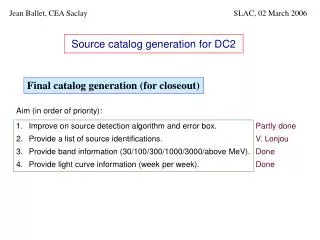
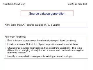
1. Source catalog generation Jean Ballet, CEA Saclay GSFC, 29 June 2005 Aim: Build the LAT source catalog (1, 3, 5 years) Four main functions: • Find unknown sources over the whole sky (output: list of positions). • Localize sources. Output: list of precise positions (and uncertainties) • Characterize sources (significance, flux, spectrum, variability). This is no different from studying already known sources, and can be done using the likelihood method. • Identify sources (find counterparts in existing external catalogs).

2. Catalog production pipeline Remove space-ground transmission artifacts Location: LAT ISOC “Pipeline” processing Level 1 Database Reconstructed events Calibration data Ancillary data LAT Raw Data Level 0 Database Raw events Interstellar model (U5) U6 U4 Location: CEA Saclay Source search List of sources Photon maps Maximum likelihood (A1) Exposure maps A2: Source identification LAT catalog (D5) List of sources and identifications List of sources Characterization Catalog Database (D6)

3. Catalog pipeline. Sequence Aim: Implement automatic loop to find and characterize the sources Minimal features: Detect sources over current diffuse model Get a precise position Run Likelihood on all sources to get precise flux, spectrum and significance Split into time pieces to get light curve Run sourceIdentify to get counterparts • Task scheduling tool (like OPUS) for distributing work over CPUs • Simple database for bookkeeping and for the source lists Associated product: sensitivity maps in several energy bands, or tool to provide minimum detectable flux as a function of spectral index and duration

4. Catalog pipeline. Schedule Identify candidate source search algorithms. Done Define evaluation criteria. Not yet concluded. Build pipeline prototype. Good progress. Evaluate candidate algorithms. Done on DC1. First selection of source search algorithm. Not done yet. Wait until DC2. Define processing database. By end 2005 Integrate pipeline elements (including flux history, identification). 2006. Ready: end 2006 (for DC3)

5. All-sky source search. Algorithms Wavelet algorithm developed at Perugia (F. Marcucci, C. Cecchi, G. Tosti) Wavelet algorithm developed at Saclay (MR_filter by J.L. Starck, presented in September 2004). On DC1, was quite comparable to 1. Optimal filter PSF/(1+BKG) in Fourier space (myself , presented in September 2004). On DC1, did not find as many sources as 1 or 2 but returns source significance. Multichromatic wavelet method developed by S. Robinson and T. Burnett. Tries using the PSF at the energy of each photon. On DC1, did not find as many sources as 1 or 2 but still interesting for localization. Aperture photometry tried by T. Stephens as a reference. On DC1, did not find as many sources as the other methods but useful exercise. Voronoi algorithm proposed by J. Scargle. Was not ready for DC1.

6. Source localization • Done locally (for each source in turn) • Typical algorithm (like SExtractor) uses a smoothed map as input, and interpolates to find the maximum. • Another possibility would be to use a different algorithm (like the multichromatic wavelet) to localize sources once they are detected. • We need to provide a precision on source position • Building TSmaps for all sources is certainly VERY CPU intensive. • The precision depends mostly on the source spectrum (estimated by likelihood) and the source significance. This can be computed once and for all, and simulations can tell whether secondary parameters (like background shape) are important.

7. Pipeline prototype • We have started with the likelihood step (most time consuming) • Basis provided by J. Chiang (catalogAnalysis package, sourceAnalysis Python script). Chains event selection, exposure map generation and likelihood run. • Use the OPUS task scheduler • Try using OPUS in a minimal way (do not decompose too much) in order to facilitate portability. • Standard region of interest (20° radius) contains many sources (several tens) • Optimizers have trouble converging over so many parameters. • Reduce area over which sources are fitted, taking nearby sources (fixed) from run on nearby region of interest. • In addition, call likelihood in several steps (first diffuse emission, then add bright sources, then add faint ones).

8. What we plan to provide at DC2 kickoff Run all-sky source detection Run likelihood over all detections of first step Provide source list (FITS format for the catalog, but not all columns will be filled) • Source_Name (just a number for internal reference), RA, Dec, Lon, Lat from all-sky source detection • Test_Statistic, Flux (> 100 MeV), Unc_Flux, Spectral_Index, Unc_Spectral_Index from likelihood What we will try to add during DC2 • Error box or ellipse • Counterparts (using sourceIdentify)

9. Source catalog generation Jean Ballet, CEA Saclay GSFC, 29 June 2005 Catalog generation is on the way ! Several open points: Should we provide fluxes in a different band (starting at higher energy than 100 MeV) to optimize the relative error ? Do we need a separate step for source localization and position error ? Should we implement additional cuts on the data (e.g. on off-axis angle) ?