Download
1 / 27
270 likes | 369 Views
Fast Switching Phase Compensation for ALMA. Mark Holdaway NRAO/ Tucson. Other Fast Switching Contributors: Frazer Owen Michael Rupen Chris Carilli Simon Radford Larry D’Addario Frank Bertoldi. At Millimeter wavelengths, The Atmosphere Messes Us Up.

E N D
Fast Switching Phase Compensation for ALMA Mark Holdaway NRAO/Tucson Other Fast Switching Contributors: Frazer Owen Michael Rupen Chris Carilli Simon Radford Larry D’Addario Frank Bertoldi URSI
At Millimeter wavelengths,The Atmosphere Messes Us Up So, we went to 5000m to escape the atmosphere! 55% of the oxygen, 5% of the water vapor Opacity: absorbs mm radiation, thermal radiation increases noise, and opacity fluctuations make calibration and imaging problematic. Phase flucuations: wrecks sensitivity – decorrelation ( e –σ2/2 ), limits image quality by putting emission in the wrong place, variable decorrelation spoils resolution (phase errors increase with baseline length) URSI
Site Testing at Chajnantor Since 1995, site monitoring has found that 230 GHz opacity is very low and often shows no diurnal effect (ie, many continuous hours of high frequency observing) URSI
Site Testing at Chajnantor Monitoring of phase errors at 11.2 GHz on a 300m baseline indicate phase errors are still a huge problem! The median phase errors on 300m baselines at 230 GHz result in 50% decorrelation loss in sensitivity if not corrected! So, lets get CORRECTING! URSI
Effective phase compensation will be required for ALMA to meet ANY science goals Fast Switching? WVR? …or a Hybrid? URSI
Effective phase compensation will be required for ALMA to meet ANY science goals Fast Switching: σφ≈√ D(d) instead of σφ≈√ D(baseline) URSI
Fast switching “cuts off” the structure function at some “effective baseline” That effective baseline is about: (v Δt+ d)/2 v = atm. vel. =10-15m/s Δt = cycle time We are dominated by the Δtterm URSI
Fast Switching Cycle can be optimized for sensitivity • Optimal calibrator minimizes (vt+d): to quantify, we need source count info • F.S. Efficiency == (e –σ2/2) ( ton / tcycle )0.5 • Over-calibrating: sensitivity lost from time • Under-calibrating: sensitivity lost from decorrelation URSI
Source counts at 90 GHz Blind Survey at 90 GHz too slow (400 sq deg down to 10 mJy) So, we target compact, flat spectrum quasars, observe at 90 GHz, determine the spectral index distribution, and scale 5GHz flat spectrum counts URSI
Source counts at higher freqs By solving for a distribution of break frequencies and assuming optically thick α~0, optically thin α~0.8, we can extrapolate to higher frequencies URSI
Source counts at 250 GHz Flat spectrum quasars observed with MAMBO as pointing sources can be used to estimate 250 GHz source counts: slightly higher than our extrapolation by fitting a break frequency distribution. URSI
What will we do at high frequencies? • At high ν, source counts decline, sensitivity declines, can’t fast switch! • Plan: calibrate at 90 GHz and scale the phase solutions by νtarget/νcal • Need an additional calibration to determine instrumental phase drifts uncommon to νtarget andνcal URSI
High Frequency Scheme: Details, such as the target sequence cycle time, can be determined through sensitivity optimization. URSI
How do we quantify the switching details? Statistical approach: • Simulate ~1000 calibrator fields, with S = f(ν) • Select the optimal calibrator: min(vt+d) • Calculate efficiency for calibrating at the target ν AND for calibrating at 90 GHz. • Results: for each band, we get a distribution of residual phase errors and a distribution of efficiencies. URSI
An example calibrator field 90 GHz 250 GHz URSI
An example distribution of fast switching efficiency Switching Efficiency: (e –σ2/2) ( ton / tcycle )0.5 URSI
Median Efficiency for several observing frequencies as a function of Phase Conditions URSI
Collapse the Distribution of Atmospheric Conditions by assuming dynamic scheduling will match high ν with high phase stability! URSI
Results (per band): • Median cal flux 50-100 mJy • Median cal time <1 s • Median slew time <1 s • Median cycle times 20-30s • Median Eff: 0.7 – 0.9 • Note: calibrating at the target frequency will be more efficient below about 300 GHz • Inst. Cal flux: 1 Jy 0.3 Jy URSI
Efficiency results factoring in atmospheric conditions and instrumental phase specification URSI
What About WVR? • Fast Switching has significant decorrelation • but: • WVR cannot solve for absolute phase, just incremental phase fluctuations • WVR cannot solve for instrumental phase, just atmospheric phase fluctuations • WVR cannot solve for any dry fluctuations URSI
Phase Calibration Hope: Instead of doing 20-30s fast switching cycles, to perform 300s switching cycles and use WVR to determine phase increments. FS can help determine the variable conversion between ΔT and Δφ. This requires that we NOT interpolate the fast switching phase solutions, and also requires that the electronic phase be fairly stable URSI
Of course, MORE WORK IS NEEDED! • Prototype antennas do meet slewing spec: 1.5deg in 1.5s • Check out fast switching interferometrically on P.I. • Start collecting information on fast switching calibrators (down to about 25 mJy – about 30,000 sources) • Understand more about the cal sources at high frequency • Observe these sources on long baselines • Simulations of WVR + Fast Switching: In progress • Keep in touch with the Software Guys URSI
After NRAO? URSI