Download

1 / 38
420 likes | 632 Views
Solid State Computing. Peter Ballo. Models. Classical: Quantum mechanical: H = E Semi-empirical methods Ab-initio methods. Molecular Mechanics. atoms = spheres bonds = springs

E N D
Solid State Computing Peter Ballo
Models • Classical: • Quantum mechanical: H = E • Semi-empirical methods • Ab-initio methods
Molecular Mechanics • atoms = spheres • bonds = springs • math of spring deformation describes bond stretching, bending, twisting Energy = E(str) + E(bend) + E(tor) + E(NBI)
From ab initio to (semi) empirical • Quantum calculation • First principles • Reliability proven within the approximations Basis sets, functional, all-electron or pseudo- potential .. • Computationally expensive • Based on fitting parameters Two body , three body…, multi-body potential • No theoretical background empirical • Applicability to large system no self consistency loop and no eigenvalue computation • Reliability ?
The Framework of DFT • DFT: the theory • Schroedinger’s equation • Hohenberg-Kohn Theorem • Kohn-Sham Theorem • Simplifying Schroedinger’s • LDA, GGA • Elements of Solid State Physics • Reciprocal space • Band structure • Plane waves • And then ? • Forces (Hellmann-Feynman theorem) • E.O., M.D., M.C. …
Using DFT • Practical Issues • Input File(s) • Output files • Configuration • K-points mesh • Pseudopotentials • Control Parameters • LDA/GGA • ‘Diagonalisation’ • Applications • Isolated molecule • Bulk • Surface
The Basic Problem Dangerously classical representation Cores Electrons
Schroedinger’s Equation Wave function Potential Energy Kinetic Energy Coulombic interaction External Fields Energy levels Hamiltonian operator Very Complex many body Problem !! (Because everything interacts)
First approximations • Adiabatic (or Born-Openheimer) • Electrons are much lighter, and faster • Decoupling in the wave function • Nuclei are treated classically • They go in the external potential
Self consistent loop Initial density From density, work out Effective potential Solve the independents K.S. =>wave functions Deduce new density from w.f. New density ‘=‘ input density ?? NO YES Finita la musica
DFT energy functional • Exchange correlation funtional • Contains: • Exchange • Correlation • Interacting part of K.E. Electrons are fermions (antisymmetric wave function)
Exchange correlation functional At this stage, the only thing we need is: Still a functional (way too many variables) • #1 approximation, Local Density Approximation: • Homogeneous electron gas • Functional becomes function !! (see KS3) • Very good parameterisation for LDA Generalised Gradient Approximation: GGA
DFT: Summary • The ground state energy depends only on the electronic density (H.K.) • One can formally replace the SE for the system by a set of SE for non-interacting electrons (K.S.) • Everything hard is dumped into Exc • Simplistic approximations of Exc work ! LDA or GGA
Bulk properties • zero temperature equations of state (bulk modulus, lattice constant, cohesive energy) • structural energy difference (FCC,HCP,BCC) • two shear elastic constants in FCC structure
M. I. Baskes, Phys. Rev. B 46, 2727 (1992) M. I. Baskes, Matter. Chem. Phys. 50, 152 (1997)
And now, for something completely different:A little bit of Solid State Physics Crystal structure Periodicity
Reciprocal space (Inverting effect) sin(k.r) Reciprocal Space bi Real Space ai Brillouin Zone k-vector (or k-point) See X-Ray diffraction for instance Also, Fourier transform and Bloch theorem
Band structure E Energy levels (eigenvalues of SE) Crystal Molecule
The k-point mesh Corresponds to a supercell 36 time bigger than the primitive cell Brillouin Zone Question: Which require a finer mesh, Metals or Insulators ?? (6x6) mesh
Plane waves • Project the wave functions on a basis set • Tricky integrals become linear algebra • Plane Wave for Solid State • Could be localised (ex: Gaussians) + + = Sum of plane waves of increasing frequency (or energy) One has to stop: Ecut
Solid State: Summary • Quantities can be calculated in the direct or reciprocal space • k-point Mesh • Plane wave basis set, Ecut
if (i.LE.n) then kx=kx-step ! Move to the Gamma point (0,0,0) ky=ky-step kz=kz-step xk=xk+step else if ((i.GT.n).AND.(i.LT.2*n)) then kx=kx+2.0*step ! Now go to the X point (1,0,0) ky=0.0 kz=0.0 xk=xk+step else if (i.EQ.2*n) then kx=1.0 ! Jump to the U,K point ky=1.0 kz=0.0 xk=xk+step else if (i.GT.2*n) then kx=kx-2.0*step ! Now go back to Gamma ky=ky-2.0*step kz=0.0 xk=xk+step end if
# Crystalline silicon : computation of the total energy # #Definition of the unit cell acell 3*10.18 # This is equivalent to 10.18 10.18 10.18 rprim 0.0 0.5 0.5 # In lessons 1 and 2, these primitive vectors 0.5 0.0 0.5 # (to be scaled by acell) were 1 0 0 0 1 0 0 0 1 0.5 0.5 0.0 # that is, the default. #Definition of the atom types ntypat 1 # There is only one type of atom znucl 14 # The keyword "znucl" refers to the atomic number of the # possible type(s) of atom. The pseudopotential(s) # mentioned in the "files" file must correspond # to the type(s) of atom. Here, the only type is Silicon. #Definition of the atoms natom 2 # There are two atoms typat 1 1 # They both are of type 1, that is, Silicon. xred # This keyword indicate that the location of the atoms # will follow, one triplet of number for each atom 0.0 0.0 0.0 # Triplet giving the REDUCED coordinate of atom 1. 1/4 1/4 1/4 # Triplet giving the REDUCED coordinate of atom 2. # Note the use of fractions (remember the limited # interpreter capabilities of ABINIT)
+ + = #Definition of the planewave basis set ecut 8.0 # Maximal kinetic energy cut-off, in Hartree #Definition of the k-point grid kptopt 1 # Option for the automatic generation of k points, taking # into account the symmetry ngkpt 2 2 2 # This is a 2x2x2 grid based on the primitive vectors nshiftk 4 # of the reciprocal space (that form a BCC lattice !), # repeated four times, with different shifts : shiftk 0.5 0.5 0.5 0.5 0.0 0.0 0.0 0.5 0.0 0.0 0.0 0.5 # In cartesian coordinates, this grid is simple cubic, and # actually corresponds to the # so-called 4x4x4 Monkhorst-Pack grid #Definition of the SCF procedure nstep 10 # Maximal number of SCF cycles toldfe 1.0d-6 # Will stop when, twice in a row, the difference # between two consecutive evaluations of total energy # differ by less than toldfe (in Hartree)
iter Etot(hartree) deltaE(h) residm vres2 diffor maxfor ETOT 1 -8.8611673348431 -8.861E+00 1.404E-03 6.305E+00 0.000E+00 0.000E+00 ETOT 2 -8.8661434670768 -4.976E-03 8.033E-07 1.677E-01 1.240E-30 1.240E-30 ETOT 3 -8.8662089742580 -6.551E-05 9.733E-07 4.402E-02 5.373E-30 4.959E-30 ETOT 4 -8.8662223695368 -1.340E-05 2.122E-08 4.605E-03 5.476E-30 5.166E-31 ETOT 5 -8.8662237078866 -1.338E-06 1.671E-08 4.634E-04 1.137E-30 6.199E-31 ETOT 6 -8.8662238907703 -1.829E-07 1.067E-09 1.326E-05 5.166E-31 5.166E-31 ETOT 7 -8.8662238959860 -5.216E-09 1.249E-10 3.283E-08 5.166E-31 0.000E+00 At SCF step 7, etot is converged : for the second time, diff in etot= 5.216E-09 < toldfe= 1.000E-06 cartesian forces (eV/Angstrom) at end: 1 0.00000000000000 0.00000000000000 0.00000000000000 2 0.00000000000000 0.00000000000000 0.00000000000000 Metals (T=0.25eV) ik=1 | eig [eV]: -5.8984 1.7993 1.9147 1.9147 2.8058 2.8058 141.3489 313.9870 313.9870 | focc: 2.0000 1.9999 1.9998 1.9998 1.9979 1.9979 0.0000 0.0000 0.0000