Transit Traffic Engineering
Transit Traffic Engineering. Nick Feamster CS 6250: Computer Networks Fall 2011. Do IP Networks Manage Themselves?. In some sense, yes: TCP senders send less traffic during congestion Routing protocols adapt to topology changes But, does the network run efficiently ?

Transit Traffic Engineering
E N D
Presentation Transcript
Transit Traffic Engineering Nick FeamsterCS 6250: Computer NetworksFall 2011
Do IP Networks Manage Themselves? • In some sense, yes: • TCP senders send less traffic during congestion • Routing protocols adapt to topology changes • But, does the network run efficiently? • Congested link when idle paths exist? • High-delay path when a low-delay path exists? • How should routing adapt to the traffic? • Avoiding congested links in the network • Satisfying application requirements (e.g., delay) • … essential questions of traffic engineering
Outline • ARPAnet routing protocols • Three protocols, with complexity/stability trade-offs • Tuning routing-protocol configuration • Tuning link weights in shortest-path routing • Tuning BGP policies on edge routers • MPLS traffic engineering • Explicit signaling of paths with sufficient resources • Constrained shortest-path first routing • Multipath load balancing • Preconfigure multiple (disjoint) paths • Dynamics adjust splitting of traffic over the path
Original ARPAnet Routing (1969) • Routing • Shortest-path routing based on link metrics • Distance-vector algorithm (i.e., Bellman-Ford) • Metrics • Instantaneous queue length plus a constant • Each node updates distance computation periodically 2 1 3 1 3 2 1 5 20 congested link
Problems With the Algorithm • Instantaneous queue length • Poor indicator of expected delay • Fluctuates widely, even at low traffic levels • Leading to routing oscillations • Distance-vector routing • Transient loops during (slow) convergence • Triggered by link weight changes, not just failures • Protocol overhead • Frequent dissemination of link metric changes • Leading to high overhead in larger topologies
New ARPAnet Routing (1979) • Averaging of the link metric over time • Old: Instantaneous delay fluctuates a lot • New: Averaging reduces the fluctuations • Link-state protocol • Old: Distance-vector path computation leads to loops • New: Link-state protocol where each router computes shortest paths based on the complete topology • Reduce frequency of updates • Old: Sending updates on each change is too much • New: Send updates if change passes a threshold
Performance of New Algorithm • Light load • Delay dominated by the constant part (transmission delay and propagation delay) • Medium load • Queuing delay is no longer negligible on all links • Moderate traffic shifts to avoid congestion • Heavy load • Very high metrics on congested links • Busy links look bad to all of the routers • All routers avoid the busy links • Routers may send packets on longer paths
I-85 SandySprings ATL GA400 “Backup at I-85”on radio triggers congestion on GA400 Over-Reacting to Congestion • Routers make decisions based on old information • Propagation delay in flooding link metrics • Thresholds applied to limit number of updates • Old information leads to bad decisions • All routers avoid the congested links • … leading to congestion on other links • … and the whole things repeats
Problem of Long Alternate Paths • Picking alternate paths • Multi-hop paths look better than a congested link • Long path chosen by one router consumes resource that other packets could have used • Leads other routers to pick other alternate paths 2 1 3 1 3 2 1 5 20 congested link
Revised ARPAnet Metric (1987) • Limit path length • Bound the value of the link metric • “This link is busy enough to go two extra hops” • Prevent over-reacting • Shed traffic from a congested link gradually • Starting with alternate paths that are just slightly longer • Through weighted average in computing the metric, and limits on the change from one period to the next • New algorithm • New way of computing the link weights • No change to link-state routing or shortest-path algorithm
2 1 3 1 3 2 1 5 4 3 Routing With “Static” Link Weights • Routers flood information to learn topology • Determine “next hop” to reach other routers… • Compute shortest paths based on link weights • Link weights configured by network operator
Setting the Link Weights • How to set the weights • Inversely proportional to link capacity? • Proportional to propagation delay? • Network-wide optimization based on traffic? 2 1 3 1 3 2 3 1 5 4 3
Measure, Model, and Control Network-wide “what if” model Topology/ Configuration Offered traffic Changes to the network measure control Operational network
Key Ingredients • Measurement • Topology: monitoring of the routing protocols • Traffic matrix: passive traffic measurement • Network-wide models • Representations of topology and traffic • “What-if” models of shortest-path routing • Network optimization • Efficient algorithms to find good configurations • Operational experience to identify constraints
Optimization Problem • Input: graph G(R,L) • R is the set of routers • L is the set of unidirectional links • cl is the capacity of link l • Input: traffic matrix • Mi,j is traffic load from routeri to j • Output: setting of the link weights • wlis weight on unidirectional link l • Pi,j,lis fraction of traffic fromito j traversing link l
0.25 0.25 0.5 1.0 1.0 0.25 0.25 0.5 0.5 0.5 Equal-Cost Multipath (ECMP) Values of Pi,j,l
f(x) x Objective Function • Computing the link utilization • Link load:ul = Si,j Mi,j Pi,j,l • Utilization: ul/cl • Objective functions • min(maxl(ul/cl)) • min(Slf(ul/cl))
Complexity of Optimization Problem • NP-complete optimization problem • No efficient algorithm to find the link weights • Even for simple objective functions • What are the implications? • Have to resort to searching through weight settings • Clearly suboptimal, but effective in practice • Fast computation of the link weights • Good performance, compared to “optimal” solution
Incorporating Operational Realities • Minimize number of changes to the network • Changing just 1 or 2 link weights is often enough • Tolerate failure of network equipment • Weights settings usually remain good after failure • … or can be fixed by changing one or two weights • Limit dependence on measurement accuracy • Good weights remain good, despite random noise • Limit frequency of changes to the weights • Joint optimization for day & night traffic matrices
Apply to Interdomain Routing • Limitations of intradomain traffic engineering • Alleviating congestion on edge links • Making use of new or upgraded edge links • Influencing choice of end-to-end path • Extra flexibility by changing BGP policies • Direct traffic toward/from certain edge links • Change the set of egress links for a destination 2 4 1 3
BGP Model for Traffic Engineering • Predict effects of changes to import policies • Inputs: routing, traffic, and configuration data • Outputs: flow of traffic through the network BGP policy configuration Topology BGP routing model BGP routes Offered traffic Flow of traffic through the network
Reasons for Interdomain TE • Congested Edge Link • Links between domains are common points of congestion in the Internet • Upgraded Link Capacity • Operators frequently install higher-bandwidth links • Aim to exploit the additional capacity • Violation of Peering Agreement
Goals for Interdomain TE • Predictable traffic flow changes • Limiting the influence of neighboring domains • Check for consistent advertisements • Use BGP policies that limit the influence of neighbors • Reduce the overhead of routing changes • Focus on small number of prefixes
Tools for Interdomain TE • Essentially, adjusting local preference to affect egress point selection • Prediction • Set of egress points per prefix • Figure out the path from each router to egress
Predictable Traffic Flow Changes • Avoid globally visible changes • Don’t do things that would result in changes to routing decisions from a neighboring AS • For example, make adjustments for prefixes that are only advertised via one neighbor AS
Limit the Influence of Neighbors • Limit the influence of AS path length • Consider treating paths that have “almost the same length” as a common group • Try to enforce consistent advertisements from neighbors (note: difficult problem!)
Reduce the Overhead of Changes • Group related prefixes • Don’t explore all combinations of prefixes • Simplify configuration changes • Routing choices: groups routes that have the same AS paths (lots of different granularities to choose from) • Focus on the (small) fraction of prefixes that carry the majority of the traffic • E.g., top 10% of origin ASes are responsible for about 82% of outbound traffic
Limitations of Shortest-Path Routing • Sub-optimal traffic engineering • Restricted to paths expressible as link weights • Limited use of multiple paths • Only equal-cost multi-path, with even splitting • Disruptions when changing the link weights • Transient packet loss and delay, and out-of-order • Slow adaptation to congestion • Network-wide re-optimization and configuration • Overhead of the management system • Collecting measurements and performing optimization
Explicit End-to-End Paths • Establish end-to-end path in advance • Learn the topology (as in link-state routing) • End host or router computes and signals a path • Routers supports virtual circuits • Signaling: install entry for each circuit at each hop • Forwarding: look up the circuit id in the table 1: 7 2: 7 1: 14 2: 8 link 7 1 link 14 2 link 8 Used in MPLS with RSVP
Label Swapping • Problem: using VC ID along the whole path • Each virtual circuit consumes a unique ID • Starts to use up all of the ID space in the network • Label swapping • Map the VC ID to a new value at each hop • Table has old ID, next link, and new ID • Allows reuse of the IDs at different links 1: 7: 20 2: 7: 53 20: 14: 78 53: 8: 42 link 7 1 link 14 2 link 8
Multi-Protocol Label Switching • Multi-Protocol • Encapsulate a data packet • Could be IP, or some other protocol (e.g., IPX) • Put an MPLS header in front of the packet • Actually, can even build a stack of labels… • Label Switching • MPLS header includes a label • Label switching between MPLS-capable routers MPLS header IP packet
Pushing Popping Swapping IP IP IP IP C A R2 R1 IP edge R4 B R3 D MPLS core Pushing, Popping, and Swapping • Pushing: add the initial “in” label • Swapping: map “in” label to “out” label • Popping: remove the “out” label
Constrained Shortest Path First • Run a link-state routing protocol • Configurable link weights • Plus other metrics like available bandwidth • Constrained shortest-path computation • Prune unwanted links (e.g., not enough bandwidth) • Compute shortest path on the remaining graph • Signal along the path • Source router sends amessage to pin thepath to destination • Revisit decisions periodically,in case better options exist 5, bw=10 s d 3, bw=80 5, bw=70 6, bw=60
Multiple Paths • Establish multiple paths in advance • To make good use of the bandwidth • To survive link and router failures
Measure Link Congestion • Disseminate link-congestion information • Flood throughout the network • Piggyback on data packets • Direct through a central controller
Adjust Traffic Splitting • Source router adjusts the traffic • Changing traffic rate or fraction on each path • … based on the level of congestion 35% 65%
Challenges • Protocol dynamics • Stability: avoid over-reacting to congestion • Convergence time: avoid under-reacting to congestion • Analysis using control or optimization theory! • Protocol overhead • State for maintaining enough (failure-disjoint) paths • Bandwidth overhead of disseminating link metrics • Computation overhead of recomputing traffic splits • Implementing non-equal traffic splitting • Hash-based splitting to prevent packet reordering • Applying the approach in an interdomain setting
Conclusion: Main Issues • How are the paths expressed? • Shortest-path routing with (changing) link weights • End-to-end path (or paths) through the network • Timescale of routing decisions? • Packet, flow, larger aggregates, longer timescale, … • Role of path diversity? • Single-path routing where the one path can be changed • Multi-path routing where splitting over paths can change • Who adapts the routes? • Routers: through adaptive routing protocols • Management system: through central (re)optimization