Download
1 / 22
250 likes | 481 Views
Another Look at Non-Rotating Origins. George Kaplan Astronomical Applications Department U.S. Naval Observatory gkaplan@usno.navy.mil. Another Look at Non-Rotating Origins Abstract.

E N D
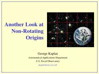
Another Look at Non-Rotating Origins George Kaplan Astronomical Applications Department U.S. Naval Observatory gkaplan@usno.navy.mil
Another Look at Non-Rotating OriginsAbstract Two “non-rotating origins” were defined by the IAU in 2000 for the measurement of Earth rotation: the Celestial Ephemeris Origin (CEO) in the ICRS and the Terrestrial Ephemeris Origin (TEO) in the ITRS. Universal Time (UT1) is now defined by an expression based on the angle between the CEO and TEO. Many previous papers, e.g., Capitaine et al. (2000), developed the position of the CEO in terms of a quantity s, the difference between two arcs on the celestial sphere. A similar quantity s was defined for the TEO. continued… IAU JD16 & Div. 1
Abstract (cont.) As an alternative, a simple vector differential equation for the position of a non-rotating origin on its reference sphere is developed here. The equation can be easily numerically integrated to high precision. This scheme directly yields the ICRS right ascension and declination of the CEO, or the ITRF longitude and latitude of the TEO, as a function of time. This simplifies the derivation of the main transformation matrix between the ITRF and the ICRS. This approach also yields a simple vector expression for apparent sidereal time. The directness of the development may have pedagogical and practical advantages for the vast majority of astronomers who are unfamiliar with the history of this topic. IAU JD16 & Div. 1
Objectives • Develop alternative mathematical description of non-rotating origins, precise enough for practical computations • Avoid spherical trig, composite arcs, etc. • Understandable to the “average astronomer” • Directly yield RA & Dec of CEO, lat and lon of TEO • Plot out path of CEO on sky and TEO on Earth • Develop corresponding rotation matrices for ITRS ICRS transformation and test “The NRO for Dummies” IAU JD16 & Div. 1
NRO Definition • Standard Given a pole P(t) and a point of origin on the equator. If O is the geocenter, then the orientation of the cartesian axes OP, O, O (where O is orthogonal to both OP and O) is determined by the condition that in any infinitesimal displacement of P there is no instantaneous rotation around OP. Then (also ) is a non-rotating origin on the moving equator. • Alternative A non-rotating origin, , is a point on the moving equator whose instantaneous motion is always orthogonal to the equator. IAU JD16 & Div. 1
ecliptic 1 1 equator of t1 2 equator of t2 2 equator of t3 3 3 Dec ICRF RA Motion of a non-rotating origin, , compared to that of the true equinox, . IAU JD16 & Div. 1
Two equators, two poles, two NROs, t apart t 0 n n0 n1 e1 x1 2 e0 O Δx x0 1 n0, n1, x0, x1 are unit vectors x1 = x0 + Δx Δx = Δz n0 where Δz is a scalar to be determined IAU JD16 & Div. 1
Differential equation for NRO position If n(t) is a unit vector toward the instantaneous pole and x(t) is a unit vector toward an instantaneous non-rotating origin, then in a few steps we get x(t) = [x(t) •n(t) ]n(t) (1) We want to obtain the path of the NRO, x(t). Note that if P, N, and F are the matrices for precession, nutation, and frame bias, then n(t) = F Pt(t) Nt(t) is the path of the pole in the ICRS . . 0 0 1 IAU JD16 & Div. 1
Numerical Integration of NRO Position, x(t) • Conceptually and practically, it is simple to integrate x(t) = [x(t) •n(t)]n(t) • Can use, for example, standard 4th-order Runge Kutta integrator • Fixed step sizes 1 day OK • Really a 1-D problem played out in 3-D, so can apply constraints at each step: |x| = 1 and x•n = 0 IAU JD16 & Div. 1
Applications of x(t) • x(t) is the path of the CEO if n(t) is the path of the CIP (celestial pole) and a proper initial point x(J2000) is selected. The path of the CIP is defined by the IAU2000A precession-nutation model, as implemented by the algorithms in the IERS Conventions (2000). The initial point, x(J2000), should be chosen to provide continuity of Earth orientation measurements on 2003 Jan 1. • x(t) is the path of the TEO if n(t) is path of terrestrial pole (xp, yp) as defined by observations and x(J2000) = 0. IAU JD16 & Div. 1
Transformations Made Easy (1 of 3) • If n(t) represents the path of the CIP (celestial pole) and x(t) represents the path of the CEO (celestial non-rotating origin), then let y = n x. The orthonormal triad x y n then represents the axes of the “intermediate frame” (equator-of-date frame with CEO as azimuthal origin) expressed ICRS coordinates • Full terrestrial-to-celestial transformation then becomes rc = CR3(-) W rt where C = ( x y n ) = (W is the polar motion matrix and R3 is a simple rotation about the z axis, which at that step is n(t).) continued... x1 y1 n1 x2 y2 n2 x3 y3 n3 (2) IAU JD16 & Div. 1
Transformations Made Easy (2 of 3) • If p represents the apparent direction of a celestial object in ICRS coordinates (its virtual place), then its azimuthal coordinate, A, in the equator-of-date frame, measured eastward from the CEO, is A = arctan ( py / px ) (3) • Its Greenwich Hour Angle (GHA), is simply GHA = A. (Here, the Greenwich meridian is defined to be the plane that passes through the TEO and the CIP axis.) continued... IAU JD16 & Div. 1
Transformations Made Easy (3 of 3) 1 0 0 • We know the position of the instantaneous (true) equinox in ICRS coordinates: (t) = F Pt(t) Nt(t) So the GHA of the true equinox — apparent sidereal time — must be simply GHA = GAST = arctan ( y / x) (4) • Need s? The node of the instantaneous equator on the ICRS equator is just N = n(t) Then s can be easily computed as the difference between the arcs x(t)Nand 0 N (0 is the ICRS origin of RA) 0 0 1 IAU JD16 & Div. 1
Does All This Work? Yes! Compare the quantity s, computed using the CEO integration scheme, with that computed using the IERS analytical formula (series). In the upper plot, the integrated and IERS curves completely overlap; the bottom plot shows the difference only a few microarcseconds. IAU JD16 & Div. 1
Long-Term CEO Position This plot shows the output of the integrator from a 50,000-year integration, using a very simple precession algorithm and no nutation. It shows the changing position of the CEO on the sky in a “fixed” (kinematically non-rotating) frame such as the ICRS. Start at J2000 approx. ecliptic This plot is similar to those previously obtained by Fukushima and Guinot from analytic developments. Note that, unlike the equinox, the CEO does not return to the same point on the sky after each precession cycle. IAU JD16 & Div. 1
Earth Orientation These plots show the difference in Earth orientation computed using the integrated CEO scheme (eq. 2) and that computed using a conventional equinox-based sidereal-time method. For sidereal time, the new IERS formula was used. The difference is only a few micro- arcseconds within two centuries of 2000. IAU JD16 & Div. 1
Earth Orientation These plots show the same difference as on the previous slide, but only IERS algorithms and parameters were used. The overall systematic pattern is obviously the same as when using the integrated CEO scheme. IAU JD16 & Div. 1
Apparent Sidereal Time This plot shows the difference between apparent sidereal time computed from the integrated CEO scheme, eq. (4), and that computed using a conventional sidereal-time formula. The new IERS formula for sidereal time was used as the “conventional” formula. Units are microarcseconds. The systematic pattern is the same as that seen previously in earth orientation RA, as one would expect. IAU JD16 & Div. 1
Earth Orientation Revisited These plots show the difference in Earth orientation computed using the integrated CEO scheme (eq. 2) and that computed using a conventional equinox-based sidereal-time method. However, for this comparison, the new Capitaine et al. (2003) formulas for precession and sidereal time were used. These appear to be more self-consistent than the IERS formulas. IAU JD16 & Div. 1
An Interesting Corollary V. Slabinski (2002, private communication) derived the NRO equation of motion (eq. 1) independently from the first definition of the NRO. He also showed that the equation implies that all NROs on a common equator must maintain constant arc distances between them. This makes sense, because we require the same rotation measurement to be obtained for all NROs. The above plot shows how well the integrator satisfies this condition. Four NROs were integrated independently, starting at year 1700 at RA=0, 1, 95, and 160, respectively. The six curves show how well the pairwise combinations maintain constant arc separations. No combination exceeds 0.5μas over 6 centuries. IAU JD16 & Div. 1
Conclusions • It is possible to provide a description of the non-rotating origin (NRO) concept that is both intuitively simple and mathematically precise • might be attractive to the broader astronomical community • The development is based on a numerical integration of an NRO position as a function of time, using an equation of motion that is simple to derive and elegant • Applied to the celestial system (ICRS), this scheme directly yields the RA and Dec of the CEO as a function of time • Terrestrial-celestial frame transformations and related algorithms become almost trivial • The results are good the numerical precision seems to be at least as good as that from the IERS algorithms IAU JD16 & Div. 1
This poster is available on the web at http://aa.usno.navy.mil/kaplan/NROs.pps or http://aa.usno.navy.mil/kaplan/NROs.pdf The text version (abridged content) submitted to the IAU Joint Discussion 16 proceedings is at http://aa.usno.navy.mil/kaplan/NROs[JD16proc].pdf George Kaplan can be contacted at the U.S. Naval Observatory at gkaplan@usno.navy.mil IAU JD16 & Div. 1