Download
1 / 56
570 likes | 590 Views
Explore the concepts of technology mapping, priority cuts, and structural choices in logic network mapping for better placement and improved performance.

E N D
Technology Mapping with Choices, Priority Cuts, and Placement-Aware Heuristics Alan Mishchenko UC Berkeley
Overview • Introduction • Technology mapping • Priority cuts • Structural choices • Tuning mapping for placement • Other applications
(1) Introduction • Terminology • And-Inverter Graphs • Technology mapping in a nutshell
Primary outputs TFO Fanouts Fanins TFI Primary inputs Root Cut Leaves Primary inputs Terminology • Logic network • Primary inputs/outputs (PIs/POs) • Logic nodes • Fanins/fanouts • Transitive fanin/fanout cone (TFI/TFO) • Structural cut of a node • Cut is a boundary in the network separating the node from the PIs • Boundary nodes are the leaves • The node is the root • K-feasible cut has K or less leaves • Function of the cut is function of the root in terms of the leaves
d a b a c b c a c b d b c a d AIG Definition and Examples AIG is a Boolean network composed of two-input ANDs and inverters. F(a,b,c,d) = ab + d(ac’+bc) 6 nodes 4 levels F(a,b,c,d) = ac’(b’d’)’ + c(a’d’)’ = ac’(b+d) + bc(a+d) 7 nodes 3 levels
f LUT LUT LUT e a c d b Primary outputs Choice node Primary inputs Mapping in a Nutshell Mapped network AIG f • AIGs reprsent logic functions • A good subject graph for mapping • Technology mapping expresses logic functions to be implemented • Uses a description of a technology • Technology • Primitives with delay, area, etc • Structural mapping • Computes a cover of AIG using primitives of the technology • Cut-based structural mapping • Computes cuts for each AIG node • Associates each cut with a primitive • Selects a cover with a minimum cost • Structural bias • Good mapping cannot be found because of the poor AIG structure • Overcoming structural bias • Need to map over a number of AIG structures (leads to choice nodes) e c d b a
(2) Technology Mapping • Traditional LUT mapping • Delay-optimal mapping • Area recovery • Drawbacks of the traditional mapping • Excessive memory and runtime • Structural bias • Ways to mitigate the drawbacks • Priority cuts • Structural choices
Traditional LUT Mapping Algorithm Input: And-Inverter Graph • Compute K-feasible cuts for each node • Compute best arrival time at each node • In topological order (from PI to PO) • Compute the depth of all cuts and choose the best one • Perform area recovery • Using area flow • Using exact local area • Chose the best cover • In reverse topological order (from PO to PI) Output: Mapped Netlist
Delay-Optimal Mapping Cut size K = 3 f • Input: • AIG and K-cuts computed for all nodes • Algorithm: • For all nodes in a topological order • Compute arrival time of each cut using fanin arrival times • Select one cut with min arrival time • Set the arrival time of the node to be the arrival time of this cut • Output: • Delay-optimal mapping for all nodes 3 Cut {pqr} of node f has arrival time 3 s r p q 1 1 2 1 a c e b d f f 2 s Cut {stu} of node f has arrival time 2 1 t u 1 1 a c e b d f
Area Recovery During Mapping • Delay-optimal mapping is performed first • Best match is assigned at each node • Some nodes are used in the mapping; others are not used • Arrival and required times are computed for all AIG nodes • Required time for all used nodes is determined • If a node is not used, its required time is set to +infinity • Slack is a difference between required time and arrival time • If a node has positive slack, its current best match can be updated to reduce the total area of mapping • This process is called area recovery • Exact area recovery is exponential in the circuit size • A number of area recovery heuristics can be used • Heuristic area recovery is iterative • Typically involved 3-5 iterations • Next, we discuss cost functions used during area recovery • They are used to decide what is the best match at each node
How to Measure Area? Suppose we use the naïve definition: Area (cut) = 1 + [ Σ area (fanin) ] (assuming that each LUT has one unit of area) y x x y p q r p q r a c e a c e b d f b d f Area of cut {pcd} = 1 + [1 + 0 + 0] = 2 Area of cut {abq} = 1 + [ 0 + 0 + 1] = 2 Naïve definition says both cuts are equally good in area Naïve definition ignores sharing due to multiple fanouts
Area-flow area-flow (cut) = 1 + [ Σ ( area-flow ( fanin ) / fanout_num( fanin ) ) ] y x x y p q r p q r a c e a c e b d f b d f Area-flow of cut {pcd} = 1 + [1 + 0 + 0] = 2 Area-flow of cut {abq} = 1 + [ 0/1 + 0/1 + ½] = 1.5 Area-flow recognizes that cut {abq} is better Area-flow “correctly” accounts for sharing (Cong ’99, Manohara-rajah ’04)
Exact Local Area Exact-local-area (cut) = 1 + [ Σ exact-local-area (fanin with no other fanout) ] f f p p 6 6 6 6 q q s s t t a b c d e f a b c d e f Cut {pef} Area flow = 1+ [(.25+.25+3)/2] = 2.75 Exact area = 1 + 0 (p is used elsewhere) Exact area will choose this cut. Cut {stq} Area flow = 1+ [.25+.25 +1] = 2.5 Exact area = 1 + 1 = 2 (due to q) Area flow will choose this cut.
Area Recovery Summary • Area recovery heuristics • Area-flow (global view) • Chooses cuts with better logic sharing • Exact local area (local view) • Minimizes the number of LUTs by looking one node at a time • The results of area recovery depends on • The order of processing nodes • The order of applying two passes • The number of iterations • Implementation details • This scheme works for the constant-delay model • Any change off the critical path does not affect critical path
Drawbacks of Traditional Mapping • Excessive memory and runtime requirements • Exhaustive cut enumeration leads to many cuts (especially when K 6) • Structural bias • The structure of the object graph does not allow good mapping to be found
Excessive Memory and Runtime • For large designs, there may be too many K-feasible cuts • 1M node AIG has ~50M 6-cuts • Requires ~2GB of storage memory and takes ~30 sec to compute • Past ways of tackling the problem • Detect and remove dominated cuts • Does not help much • Perform cut pruning (store N cuts/node) • Throws away useful cuts even if N = 1000 • Store only cuts on the frontier • Reduces memory but increases runtime
Structural Bias • Consider mapping 4:1 MUX into 4-LUTs • The naïve approach results in 3 LUTs • After logic structuring, mapping with 2 LUTs can be found
Ways to Mitigate the Drawbacks • Excessive memory and runtime requirements • Compute only a small number of “useful” cuts • Leads to mapping with priority cuts • Structural bias • Perform mapping over multiple circuit structures • Leads to mapping with structural choices
(3) Priority Cuts • Structural cuts • Exhaustive cut enumeration • Prioritizing cuts • Implementation tricks
Structural Cuts in AIG n A cutof a node n is a set of nodes in transitive fanin such that every path from the node to PIs is blocked by nodes in the cut. A k-feasible cut has no more than k leaves. p q a b c The set {pbc} is a 3-feasible cut of node n. (It is also a 4-feasible cut.) k-feasible cuts are important in LUT mapping because the logic between root n and the cut leaves {pbc} can be replaced by a k-LUT.
{ n,pq, pbc, abq, abc } n { p,ab} { q,bc } p q { b } { c } { a } a c b Exhaustive Cut Enumeration Computation is done bottom-up The set of cuts of a node is a ‘cross product’ of the sets of cuts of its children. Any cut that is of size greater than k is discarded. (P. Pan et al, FPGA ’98; J. Cong et al, FPGA ’99)
Cut Filtering Bottom-up cut computation in the presence of re-convergence might produce dominated cuts x { .. {adbc} .. {abc} .. } f { .. {dbc} .. {abc} .. } d e Cut {a, b, c} dominates cut {a, d, b, c} a b c • The “good” cut {abc} is present (so not a quality issue) • But the “bad” cut {adbc} may be propagated further (so a run-time issue) • It is important to discard dominated cuts quickly
sig (c) = Σ 2ID(n) mod 32 nÎc Signature-Based Cut Filtering Problem: Given two cuts, how to quickly determine whether one can be a subset of another. Solution: Signature of a cut is a 32-bit integer defined as: (Σ means bit-wise OR) where ID(n) is the integer id of node n Observation: If cut c1 dominates cut c2, then sig(c1) OR sig(c2) = sig(c2) Signature checking is a quick test for the most common case when a cut does not dominate another. Only if this check fails, an actual comparison is performed.
Example • Let the node IDs be a = 1, b = 2, c = 3, d= 4 • Let c1 = {a, b, c} and c2 = {a, d, b, c} • sig (c1) = 21OR 22OR 23 = 0001 OR 0010 OR 0100 = 0111 • sig (c2) = 21OR 24OR 22OR 23 = 0001 OR 1000 OR 0010 OR 0100 = 1111 • As sig (c1) OR sig (c2) ¹ sig (c1), c2 does not dominate c1 • But sig (c1) OR sig (c2) = sig (c2), so c1may dominate c2
Experiment with K-Cut Computation C/N is the number of cuts per node; T is time in seconds; L/N is the ratio of nodes with the number of cuts exceeding the limit (N=1000); for K < 8, the number of cuts did not exceed 1000
Computing Priority Cuts • Consider nodes in a topological order • At each node, merge two sets of fanin cuts (each containing C cuts) resulting in (C+1) * (C+1) + 1 cuts • Sort these cuts using a given cost function, select C best cuts, and use them for computing priority cuts of the fanouts • Select one best cut, and use it to map the node • Sorting criteria The tie-breaking criterion denoted “fanin refs” means “prefer cuts with larger average fanin reference counters”.
Priority Cuts: A Bag of Tricks • Compute and use priority cuts (a subset of all cuts) • Dynamically update the cuts in each mapping pass • Use different sorting criteria in each mapping pass • Include the best cut from the previous pass into the set of candidate cuts of the current pass • Consider several depth-oriented mappings to get a good starting point for area recovery • Use complementary heuristics for area recovery • Perform cut expansion as part of area recovery • Use efficient memory management
Priority-Cut-Based Mapping Input: And-Inverter Graph • Compute K-feasible cuts for each node • Compute arrival time at each node • In topological order (from PI to PO) • Compute the depth of all cuts and choose the best one • Compute at most C good cuts and choose the best one • Perform area recovery • Using area flow • Using exact local area • In each iteration, re-compute at most C good cuts and choose the best one • Chose the best cover • In reverse topological order (from PO to PI) Output: Mapped Netlist
Complexity Analysis • The worst-case complexity of traditional mapping • FlowMap O(Kmn) (J. Cong et al, TCAD ’94) • CutMap O(2KmnK) (J. Cong et al, FPGA ’95) • DAOmap O(KnK) (J. Cong et al, ICCAD’04) • Mapping with priority cuts • O(KC2n) K is max cut size C is max number of cuts n is number of nodes m is number of edges
(4) Structural Choices • Structural bias • Ways to overcome structural bias • Need some form of (re)synthesis to get multiple circuit structures • Computing and using several synthesis snapshots • Running several scripts and combining the resulting networks • Performing Boolean decomposition during mapping • Multiple circuit structures = structural choices • Questions: • How to efficiently detect and store structural choices? • How to perform technology mapping with structural choices?
Structural Bias The mapped netlist very closely resembles the subject graph f f p LUT p Technology Mapping LUT m m LUT e e a c d a c d b b Every input of every LUT in the mapped netlist must be present in the subject graph - otherwise technology mapping will not find the match
Example of Structural Bias A better match may not be found f f This match is not found p LUT p f LUT LUT q m m LUT LUT a e e b c e a c d a c d d b b Since the point q is notpresent in the subject graph, the match on the right is notfound
f p m e a c d b Example of Structural Bias The better match can be found with a different subject graph f p f synthesis LUT q q LUT a b c e d a c d b e
Synthesis for Structural Choices • Traditional synthesis produces one “optimized” network • Synthesis with choices produces several networks • These can be different snapshot of the same synthesis flow • These can be results of synthesizing the design with different options • For example, area-oriented and delay-oriented scripts Synthesis D1 D2 D3 D4 Synthesis with structural choices D1 D4 HAIG D2 D3
Mapping with Structural Choices • Two questions have to be answered • How to store multiple circuit structures? • How to perform mapping with multiple circuit structures? • Both questions can be solved due to the following: • The subject graph is an AIG • Structural hashing quickly merges isomorphic circuit structures • There are powerful equivalence checking methods • They can be used to prove equivalence • Cut computation can be extended to work with structural choices • The modification is straight-forward
Detecting Choices Given two Boolean networks, create a network with choices Network 1 x = (a + b)c y = bcd Network 2 x = ac + bc y = bcd Step 1: Make And-Inverter decomposition of networks y y x x a c d a c d b b
Detecting Choices Step 2: Use combinational equivalence to detect functionally equivalent nodes up to complementation (A. Kuehlmann, TCAD’02) • Random simulation to detect possibly equivalent nodes • SAT-based decision procedure to prove equivalence Network 1 x = (a + b)c y = bcd Network 2 x = ac + bc y = bcd x y y x a c d a c d b b
y x a c d b Detecting Choices Step 3: Merge equivalent nodes with choice edges x y a c d b x y x now represents a class of nodes that are functionally equivalent up to complementation a c d b
Cut Computation with Choices Cuts are now computed for equivalence classes of nodes { x1, pr, pbc, acr, abc } { x2, qc, abc } x y x1 x2 r p q a c d b Cuts ( x ) = Cuts ( x1 ) Cuts( x2 ) = { x1, pr, pbc, acr, abc,x2, qc }
Mapping Algorithm with Choices Only Step 1 has to be changed Input: And-Inverter Graph with choices • Compute K-feasible cuts with choices • Compute best arrival time at each node • In topological order (from PI to PO) • Compute the depth of all cuts and choose the best one • Perform area recovery • Using area flow • Using exact local area • Chose the best cover • In reverse topological order (from PO to PI) Output: Mapped Netlist
(5) Tuning Mapping for Placement • Placement-aware cost function for priority-cut computation • The total number of edges in a mapped network • Advantages • Correlates with the total wire-length after placement • Easy to take into account during area recovery • Treat “edges” as “area” resulting in • Edge flow (similar to area flow) • Exact local edges (similar to exact local area) • WireMap • New placement-aware mapping algorithm
Modified Cut Prioritization Heuristics in WireMap • Consider nodes in a topological order • At each node, merge two sets of fanin cuts (each containing C cuts) getting (C+1) * (C+1) + 1 cuts • Sort these cuts using a given cost function, select C best cuts, and use them for computing priority cuts of the fanouts • Select one best cut, and use it to map the node • Sorting criteria
WireMap Algorithm Input: And-Inverter Graph • Compute K-feasible cuts for each node • Compute best arrival time at each node • In topological order (from PI to PO) • Compute the depth of all cuts and choose the best one • Perform area recovery • Using area flow and edge flow • Using exact local area and exact local edge • Chose the best cover • In reverse topological order (from PO to PI) Output: Mapped Netlist
Experimental Results • Experimental comparison • WireMap vs. the same mapper w/o edge heuristics • WireMap leads to the average edge reduction • 9.3% (while maintaining depth and LUT count) • Place-and-route after WireMap leads to • 8.5% reduction in the total wire length • 6.0% reduction in minimum channel width • 2.3% reduction in critical path delay • Changes in the LUT size distribution • The ratio of 5- and 6-LUTs in a typical design is reduced • The ratio of 2-, 3-, and 4-LUTs is increased • Changes after LUT merging • 9.4% reduction in dual-output LUTs
(6) Other Applications of Priority-Cut-Based Mapping • Sequential mapping (mapping + retiming) • Speeding up SAT solving • Cut sweeping • Delay-oriented resynthesis for sequential circuits
Sequential Mapping • That is, combinational mapping and retiming combined • Minimizes clock period in the combined solution space • Previous work: • Pan et al, FPGA’98 • Cong et al, TCAD’98 • Our contribution: dividing sequential mapping into steps • Finding the best clock period via sequential arrival time computation (Pan et al, FPGA’98) • Running combinational mapping with the resulting arrival/required times of the register outputs/inputs • Performing final retiming to bring the circuit to the best clock period computed in Step 1
Sequential Mapping (continued) • Advantages • Uses priority cuts (L=1) for computing sequential arrival times • very fast • Reuses efficient area recovery available in combinational mapping • almost no degradation in LUT count and register count • Greatly simplifies implementation • due to not computing sequential cuts (cuts crossing register boundary) • Quality of results • Leads to ~15% better quality compared to comb. mapping + retiming • due to searching the combined search space • Achieves almost the same (-1%) clock period as the general sequential mapping with sequential cuts • due to using transparent register boundary without sequential cuts
Speeding Up SAT Solving • Perform technology mapping into K-LUTs for area • Define area as the number of CNF clauses needed to represent the Boolean function of the cut • Run several iterations of area recovery • Reduces the number of CNF clauses by ~50% • Compared to a good circuit-to-CNF translation (M. Velev) • Improves SAT solver runtime by 3-10x • Experimental results are in the SAT’07 paper
Cut Sweeping • Reduce the circuit by detecting and merging shallow equivalences (proposed by Niklas Een) • By “shallow” equivalences, we mean equivalent points, A and B, for which there exists a K-cut C (K < 16) such that FA(C) = FB(C) • A subset of “good” K-cuts can be computed • The cost function is the average fanout count of cut leaves • The more fanouts, the more likely the cut is common for two nodes • Cut sweeping quickly reduces the circuit • Typically ~50% gain of SAT sweeping (fraiging) • Cut sweeping is much faster than SAT sweeping • Typically 10-100x, for large designs • Can be used as a fast preprocessing to (or a low-cost substitute for) SAT sweeping
Sequential Resynthesis for Delay • Restructure logic along the tightest sequential loops to reduce delay after retiming (Soviani/Edwards, TCAD’07) • Similar to sequential mapping • Computes seq. arrival times for the circuit • Uses the current logic structure, as well as logic structure, transformed using Shannon expansion w.r.t. the latest variables • Accepts transforms leading to delay reduction • In the end, retimes to the best clock period • The improvement is 7-60% in delay with 1-12% area degradation (ISCAS circuits) • This algorithm could benefit from the use of priority cuts