Download
1 / 49
490 likes | 601 Views
X-ray clusters and cosmology. In collaboration with:. Steve Allen, KIPAC. David Rapetti (KIPAC) Adam Mantz (KIPAC) Harald Ebeling (Hawaii) Robert Schmidt (Heidelberg) R. Glenn Morris (KIPAC) Andy Fabian (Cambridge). Why study clusters at X-ray wavelengths?.

E N D
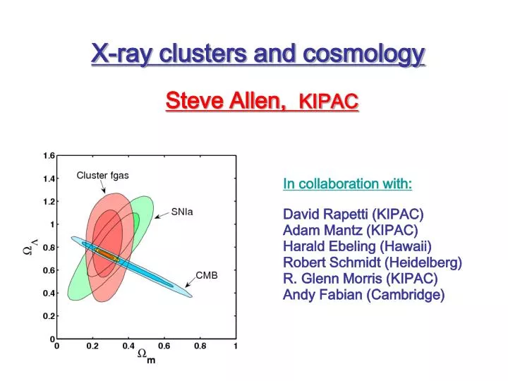
X-ray clusters and cosmology In collaboration with: Steve Allen, KIPAC David Rapetti (KIPAC) Adam Mantz (KIPAC) Harald Ebeling (Hawaii) Robert Schmidt (Heidelberg) R. Glenn Morris (KIPAC) Andy Fabian (Cambridge)
Why study clusters at X-ray wavelengths? Most baryons in clusters (like Universe) are in form of gas, not stars (6x more). In clusters, gravity squeezes gas, heating it to X-ray temperatures (107-108 K) Since clusters only shine in X-rays if they really are massive, X-ray observations produce remarkably clean cluster catalogues, vital for cosmology. Primary X-ray observables (density, temperature) relate directly to total (dark plus luminous) mass in a way that’s well understood (hydrostatic equilibrium) and can be well modelled by hydro. simulations.
Outline of the talk 1) Constraints onthe mean matter density Ωm and dark energy (Ωde,w) from measurements of the baryonic mass fraction in the largest dynamically relaxed clusters [distance measurements]. 2) Constraints onthe mean matter density Ωm, the amplitude of matter fluctuations 8, and dark energy (Ωde,w), from the evolution of the number density of X-ray luminous clusters [growth of cosmic structure]. + a little on what these tests can do in combination.
Probing cosmology with X-ray clusters 1. The fgas experiment Allen et al. 2008, MNRAS, 383, 879 (See also White & Frenk ’91; Fabian ’91; Briel et al. ’92; White et al ’93; David et al. ’95; White & Fabian ’95; Evrard ’97; Mohr et al ’99; Ettori & Fabian ’99; Roussel et al. ’00; Grego et al ’00; Ettori et al. ’03; Sanderson et al. ’03; Lin et al. ’03; LaRoque et al. ’06; Allen et al. ’02, ’03, ’04.)
The Chandra data 42 hot (kT>5keV), highly X-ray luminous (LX>1045 h70-2 erg/s), dynamically relaxed clusters spanning redshifts 0<z<1.1 (lookback time of 8Gyr) Regular X-ray morphology: sharp central X-ray surface brightness peak, minimal X-ray isophote centroid variation, low power-ratios (morphological selection).
Constraining Ωmwith fgas measurements BASIC IDEA (White & Frenk 1991): Galaxy clusters are so large that their matter content should provide a fair sample of matter content of Universe. For relaxed clusters: X-ray data good total mass measurements precise X-ray gas mass measurements eg Lin & Mohr 04 Fukugita et al ‘98 If we define: Then: Since clusters provide ~ fair sample of Universefbaryon=bΩb/Ωm
The measured fgas values depend upon assumed distances to clustersfgasd 1.5. This introduces apparent systematic variations in fgas(z) depending on differences between reference cosmology and true cosmology. • Constraining dark energy with fgas measurements What do we expect to observe? Simulations: (non-radiative) For large (kT>5keV) relaxed clusters simulations suggest little evolution of depletion factor b(z) within z<1. So we expect the observed fgas(z) values to be approx. constant with z. Precise prediction of b(z) is a key task for new hydro. simulations.
SCDM (Ωm=1.0, ΩΛ=0.0) ΛCDM (Ωm=0.3, ΩΛ=0.7) • Chandra results on fgas(z) Brute-force determination of fgas(z) for two reference cosmologies: Inspection clearly favours ΛCDM over SCDM cosmology.
To quantify: fit data with model which accounts for apparent variation in fgas(z) as underlying cosmology is varied → find best fit cosmology.
Our full analysis includes a comprehensive and conservativetreatment of potential sources of systematic uncertainty in current analysis. • Allowances for systematic uncertainties 1) The depletion factor (simulation physics, gas clumping etc.) b(z)=b0(1+bz) 20% uniform prior on b0 (simulation physics) 10% uniform prior on b (simulation physics) 2) Baryonic mass in stars: define s= fstar/fgas =0.16h700.5 s(z)=s0(1+sz) 30% Gaussian uncertainty in s0 (observational uncertainty) 20% uniform prior on s (observational uncertainty) 3) Non-thermal pressure support in gas: (primarily bulk motions) = Mtrue/MX-ray 10% (standard) or 20% (weak) uniform prior 1<<1.2 4) Instrument calibration, X-ray modelling K 10% Gaussian uncertainty
With these (conservative) allowances for systematics Model: Results (ΛCDM) Full allowance for systematics + standard priors: (Ωbh2=0.0214±0.0020, h=0.72±0.08) Best-fit parameters (ΛCDM): Ωm=0.27±0.06,ΩΛ=0.86±0.19 (Note also good fit:2=41.5/40) Important
The low systematic scatter in the fgas(z) data The 2 value is acceptable even though rms scatter about the best-fit model is only 15% in fgas, or 10% in distance. Weighted-mean scatter only 7.2% in fgas or 4.8% in distance). c.f. SNIa, for which systematic scatter detected at ~7% level (distance). Consistent with expectation from simulations (e.g. Nagai et al. ’07) The low systematic scatter in fgas(z) data offers the prospect to probe cosmic acceleration to high precision using the next generation of X-ray observatories e.g. Constellation-X (Rapetti & Allen, astro-ph/0710.0440).
Comparison of independent constraints (ΛCDM) fgas analysis: 42 clusters including standard Ωbh2, and h priors and full systematic allowances CMB data (WMAP-3yr +CBI+ACBAR + prior 0.2<h<2.0) Supernovae data from Davis et al. ’07 (192 SNIa, ESSENCE+ SNLS+HST+nearby). Combined constraint (68%) Ωm = 0.275 ± 0.033 Ω= 0.735 ± 0.023 Allen et al 2008
Ωm = 0.253 ± 0.021 w0 = -0.98 ± 0.07 • Dark energy equation of state: Constant w model: Analysis assumes flat prior. 68.3, 95.4% confidence limits for all three data sets consistent with each other. Combined constraints (68%) Note: combination with CMB data removes the need for Ωbh2 and h priors.
Results for evolving equation of state (flat prior) Free transition redshift: Allow 0.5<1/(1+zt)<0.95. Marginalized constraints (68%) w0 = -1.05 (+0.31,-0.26) wet =-0.83 (+0.48,-0.43) Conclude: fgas+CMB+SNIa data consistent with cosmological constant model.
Relaxing the flat prior (constant w model) Due to the complementary nature of the fgas+CMB+SNIa data, one can drop the assumption of ΩK=0 in the analysis and still obtain tight constraints on DE. Marginalized constraints (68%) ΩM = 0.278 (+0.064, -0.050) ΩDE = 0.732 (+0.040, -0.046) w0 = -1.08 (+0.13, -0.19) ΩK = -0.011 (+0.015, -0.017)
Probing cosmology with X-ray clusters 2. The growth of cosmic structure (evolution of the XLF) Mantz et al. 2008, MNRAS, in press (astro-ph/0709.4294) (See also e.g. Borgani et al ’01; Reiprich & Bohringer ’02; Seljak ’02; Viana et al ’02; Allen et al. ’03; Pierpaoli et al. ’03; Vikhlinin et al. ’03; Schuecker et al ’03; Voevodkin & Vikhlinin ’04; Henry ’04; Dahle ’06 etc.)
Moore et al. Borgani ‘06 • Cluster growth of structure experiments The observed growth rate of galaxy clusters provides (highly) complementary constraints on dark matter and dark energy to those from distance measurements.
[THEORY] The predicted mass function for clusters, n(M,z), as a function of cosmological parameters (8,m,w0, wa etc) in hand from current + near future numerical simulations (e.g. Jenkins et al. ’01) • Ingredients for cluster growth of structure experiments [CLUSTER SURVEY] A large, wide-area, clean, complete cluster survey, with a well defined selection function. Current leading work based on ROSAT X-ray surveys. Future important work based on new SZ (SPT, Planck) and optical catalogues as well as next-generation X-ray surveys (eROSITA/WFXT). [SCALING RELATION]A tight, well-determined scaling relation between survey observable (e.g. Lx) and mass, with minimal intrinsic scatter.
BCS (Ebeling et al. ’98, ’00) Fx>4.4×10⁻¹²ergcm-2s-1 . 78 clusters above Lx limit. REFLEX (Bohringer et al ’04). Fx>3.0×10⁻¹²ergcm-2s-1 . 130 clusters above Lx limit. MACS (Ebeling et al. ’01, ’07) Fx>2.0×10⁻¹² ergcm-2s-1 . 36 clusters above Lx limit. • The BCS, REFLEX and MACS X-ray survey data 244 clusters with Lx > 2.55x1044 h70-2 erg s-1 To minimize systematic uncertainties, our analysis is limited to most massive, most X-ray luminous clusters with Lx > 2.55x1044 h70-2 erg s-1 (dashed line)
Reiprich & Bohringer ‘02 Nagai et al ‘07 • Scaling relation: X-ray luminosity and mass (use data at z<0.1) M,L both from X-ray observations. Major uncertainty is scale of bulk/turbulent motions in X-ray emitting gas. Can correct for this using hydro. simulations. Based on sims assume bias -25(±5)% and scatter ±15(±3)% due to bulk motions. Alternatively, can measure masses via gravitational lensing. Independent method with very different uncertainties. Work on this is underway….
Take log with • Fitting the mass-luminosity data Note: includes allowance for non-similar evolution. We extrapolate measured masses to Mvir using NFW model with appropriate range of `concentration’. Use modified chi-square to associate goodness-of-fit with M-L parameters in presence of intrinsic scatter. fixed to give best-fit reduced chi-square ~1. Estimated log-normal intrinsic dispersion in luminosity for a given mass.
Fitted model parameters:h, bh2, ch2, 8, ns, w, A, , , , 0, 1,B. • Cosmological analysis Log likelihood with (M-L goodness of fit), (2nd term penalizes models for which measured intrinsic dispersion in mass-luminosity relation, , is different from model dispersion, ) and true luminosity, detected luminosity, predicted no. density, with
Our full analysis includes the following priors and conservative allowances for systematic uncertainties: • Priors and allowances for systematic uncertainties 1) Cosmological parameters (not needed if CMB data employed) Hubble constant, h 0.72±0.08 (standard), 0.72±0.24 (weak) baryon density, bh2 0.0214±0.0020 (standard), 0.0214±0.0060 (weak) spectral index, ns 0.95 fixed (standard), 0.9<ns<1.0 (weak) 2) Jenkins mass function normalization, A ±20% (standard), ±40% (weak) 3) Mass-luminosity relation non-thermal pressure support 25±5% (standard), 25±10% (weak) non-thermal pressure scatter 15±3% (standard), 15±6% (weak), evolution of M-L scatter±20% uniform (standard), ±40% (weak) non-self similar M-L evolution ±20% uniform (standard), ±40% (weak)
Ωm = 0.28 (+0.11, -0.07) 8 = 0.78 (+0.11,-0.13) BCS: Ωm = 0.26 (+0.25, -0.09) 8 = 0.78 (+0.10, -0.37) • Results on 8, m (flat CDM model) REFLEX: Ωm = 0.20 (+0.10,-0.04) 8 = 0.85 (+0.10, -0.09) MACS: Ωm = 0.30 (+0.24, -0.10) 8 = 0.73 (+0.14, -0.13) all Combined constraints (68%) Mantz et al 2008
Flat CDM model: • Comparison with best other current results on 8, m X-ray cluster number counts (Mantz et al. ’08; this study) CMB data (WMAP3) Cosmic Shear (weak lensing) 100 square degree survey (Benjamin et al. ’07) 68.3, 95.4% confidence limits shown in all cases. Good agreement between results from 3 independent astrophysical methods
Ωm = 0.24 (+0.15, -0.07) 8 = 0.85 (+0.13, -0.20) w = -1.4 (+0.4,-0.7) Flat, constant w model: REFLEX+BCS+MACS (z<0.7). 242 clusters, Lx>2.55e44 erg/s. 2/3 sky. n(M,z) only. 68.3, 95.4% confidence limits • Results on dark energy Marginalized constraints (68%) First constraint on w from a cluster growth of structure experiment
Flat, constant w model: • Comparison with best other constraints on dark energy X-ray cluster number counts (Mantz et al. ’08) X-ray cluster fgas analysis (Allen et al ’08) CMB data (WMAP-3yr) (Spergel et al ‘07) SNIa data (Davis et al. ’07 (192 SNIa, ESSENCE+ SNLS+HST+nearby). Good agreement between all 4 completely independent techniques. All data sets independently consistent with cosmological constant (w = -1) model.
Flat, constant w model: • Combined constraint on dark energy XLF+fgas+WMAP3+SNIa Marginalized constraints (68%) Ωm = 0.269±0.016 8 = 0.82±0.03 w = -1.02±0.06 Combined constraint consistent with cosmological constant to 6% precision.
fgas(z) data for largest relaxed clusters tight constraints on ΩM, Ωand w via absolute distance measurements. • ΩM=0.27±0.06ΩΛ=0.86±0.19 (w= -1.14±0.31) • Conclusions • Measurements of the growth of X-ray luminous clusters spanning 0<z<0.7 independent constraints on ΩM,8 and w. • ΩM=0.28(+0.11,-0.07)8=0.78(+0.11,-0.13) (w= -1.4 +0.4,-0.7) • The combination of X-ray growth of structure, fgas, CMB and SNIa data already constrain dark energy to be consistent with cosmological constant at 6% level. • ΩM=0.269±0.0168=0.82±0.03 w= -1.02±0.06 • Immediate next steps (current data): explore implications for dark energy vs. modified gravity models, species-summed neutrino mass etc. • Future: more X-ray data, gravitational lensing studies (M-L), improved hydro. simulations, new X-ray/SZ surveys, Constellation-X/XEUS.
Further checks for systematics in the fgas experiment
Comparison of observed and simulated fgas profiles Good agreement with non-radiative sims. Blue: Chandra data Red: relaxed simulated Green: unrelaxed simulated New large hydro. simulations, constrained to match X-ray+optical observations, should significantly reduce uncertainties b(z) improved constraints.
Checks on hydrostatic assumption 1 X-ray pressure maps: (from projected kT and emission measure) MS2137-2353 (z=0.313) 40x1e3 counts A2029 (z=0.078) 100x1e4 counts (Million et al., in preparation) X-ray pressure maps can reveal departures from hydrostatic equilibrium. Analysis confirms dynamically relaxed nature of target clusters.
Checks on hydrostatic assumption 2 Gravitational lensing: provides an independent way to measure cluster masses that is independent of the dynamical state of the matter . Ambitious lensing study underway (with A. von der Linden, D. Applegate, P. Kelly, M. Bradac, M. Allen, G. Morris, D. Burke, P. Burchat, H. Ebeling): 50+ clusters with deep, multi-color Subaru+HST+spectroscopic data (in progress). Also work by other groups. Initial findings by Mahdavi et al. (2008) suggests little systematic offset between X-ray and lensing masses measured within r2500 on average. M2500X See also Bradac et al 2008, ApJ, in press (astro-ph/0711.4850) M2500L
A systematic trend of fgas with temperature? We find no evidence for a trend of fgas with kT in the Chandra data for kT>5keV. Best-fit power-law model is consistent with a constant. (plot shows 2-sigma limits).
Marginalized results on dark energy (ΛCDM) Blue: standard priors on Ωbh2,h. ΩΛ= 0.86±0.19 Red: weak (3x) priors on Ωbh2, h. ΩΛ= 0.86±0.21 (99.99% significance detection, comparable precision to best current SNIa studies combined) Like SNIa studies, fgas(z) data measure d(z) directly andshow Universe is accelerating. Note astrophysics relatively simple and very different from SNIa.
Exploring the sensitivity to priors, scatter and systematic allowances in the XLF analysis
flat, constant w • Effects of relaxing the priors (ns) Black solid: standard priors (ns=0.95) Blue dash: weak priors(0.9<ns<1.0) Conclusions: results relatively insensitive to prior on ns
flat, constant w • Effects of relaxing the priors (bh2, h) Black solid: standard priors Blue dash: weak priors (tripple) Conclusions: results relatively insensitive to priors on bh2, h.
flat, constant w • Effects of relaxing the priors (self-similar evolution) Black solid: standard priors (20%) Blue dash: weak priors (40%) Conclusions: results relatively insensitive to prior on .
flat, constant w • Effects of ignoring scatter (Poisson errors: survey fluxes) Black solid: standard analysis Blue dash:ignore Poisson errors Conclusions: some shift in 8, m significant underestimation of uncertainties.
flat, constant w • Effects of ignoring scatter (intrinsic M-Lx scatter) Black solid: standard analysis Blue dash:=0 (zero scatter) Conclusions: some shift in 8, m significant underestimation of uncertainties
flat, constant w • Correction for non-thermal pressure support Black solid: standard analysis (25±5% correction) Blue dash: no correction for non-thermal pressure Conclusions: significant shift in 8 significant underestimation of uncertainties
Hydro simulations of X-ray clusters Nagai, Vikhlinin & Kravtsov ‘07 Large, independent programs have been undertaken to simulate X-ray observations of clusters using state-of-the-art hydro codes and selecting/ analysing these systems in an identical manner to real observations. The most recent results have provided good news for X-ray cluster cosmology: systematics are moderate-to-small and can be quantified.
X-ray gas mass to ~1% accuracy. Total mass and fgas to several % accuracy (both bias and scatter). For relaxed clusters, X-ray studies precise masses Nagai, Vikhlinin & Kravtsov ‘07 For largest, relaxed clusters (selected on X-ray morphology) at r2500 we expect to measure: Primary uncertainty (beyond innermost core) is residual bulk motions in gas. Relaxed clusters (filled circles)
X-ray gas mass to ~1% accuracy. Total mass to several % accuracy (both bias and scatter). For unrelaxed clusters corrections required Nagai, Vikhlinin & Kravtsov ‘07 For largest, relaxed clusters (selected on X-ray morphology) at r2500 we expect to measure: Primary uncertainty (beyond innermost core) is residual bulk motions in gas. For general cluster population and larger measurement radius (r500): Corrections of 20-30% to total mass measurements from X-rays required. Relaxed clusters (filled circles)
X-ray observables correlate tightly with mass Kravtsov, Nagai, Vikhlinin ‘06 -The correlations are tight and independent of the background cosmology. -Good match to observations (at least beyond innermost core)
Low-redshifts (z<0.3): ROSAT Brightest Cluster Sample(BCS: Ebeling et al. ’98, ’00). Based on RASS (northern sky). 201 clusters with Fx>4.4x10⁻¹² erg cm-2 s-1 (0.1-2.4keV). 78 massive clusters with Lx>2.55x1044h70-2erg s-1. ~100% complete. • Current best cluster surveys in X-rays REFLEX (Bohringer et al ’04). Based on RASS (southern sky). 447 clusters with Fx>3.0x10⁻¹² erg cm-2 s-1 (0.1-2.4keV). 130 massive clusters with Lx>2.55x1044h70-2erg s-1 and Fx>3.0x10⁻¹² erg cm-2 s-1. ~100% complete. Intermediate redshifts (0.3<z<0.7): MACS (Ebeling et al ’01,’07). Based on RASS (whole sky: 23000 sq. deg). 124 clusters with Fx>10-12 erg cm-2 s-1 (0.1-2.4keV). 36 massive clusters with Fx>2.0x10⁻¹² erg cm-2 s-1 and Lx>2.55x1044h70-2erg s-1. ~100% complete. *Also note ROSAT 400 sq. degree survey (Vikhlinin et al ’08). ROSAT serendipitous cluster catalogue. 266 groups/clusters with Fx>1.4x10⁻¹³ erg cm-2 s-1.(100% redshift complete).